Have you ever wondered why the optimization community and the Bayesian community—two fundamental areas of machine learning—have so little in common? When you realize how important they are to machine learning, you start to wonder why they seem so detached from each other. Perhaps it has to do with the origins of the fields, where one comes from applied math and the other comes from statistics. In this post, I’ll talk about The Bayesian Learning Rule (Khan & Rue, 2023), a recent research direction that makes the connection between the two fields principled, clear, and practical under an elegant variational learning framework.

[Note: This is a long post. You can skim through it to get a sense.]

Bayesian methods have long been celebrated for their ability to explain various phenomena in science and solve numerous problems within a single modeling framework. However, while the post-hoc explanatory¹ power of Bayesian inference is impressive, it can sometimes be overemphasized and may not always translate effectively to practical applications, particularly in areas like deep learning. Nevertheless, it has consistently proven itself to be a powerful modeling tool, offering comprehensive views by bridging results from distinct domains and analyzing them using the same tools. In science, connections that elegantly unify two seemingly disparate concepts are highly valuable because they simplify things and complete the picture. A unified framework offers a vantage point to explore what lies beyond its components, leading to new insights and breakthroughs. This is exemplified by physicists’ desire for a theory of everything. Similarly, in machine learning, a unified perspective helps us identify the next frontiers to explore.

This post introduces such a connection between Bayes and optimization, reminiscent of the link between ridge regression and the maximum a posteriori estimator given a Gaussian prior, but applicable in a much broader context (and useful for deep learning, too). The main ingredients of this connection are the natural gradient descent (Amari, 1998, Martens, 2020) and the exponential family of distributions, which together provide a versatile rule that can derive many known, practical algorithms using standard approximations. This rule is called the Bayesian Learning Rule (BLR) (Khan & Rue, 2023), which will be the main focus of this post.

The first section is a casual introduction to gradient descent (the one we all know and love) and mirror descent (the hero in disguise), which can be skipped if the reader knows enough about them. This will serve as a motivation and will give some intuition for the next section, which is about an information-theoretic objective that reformulates the optimization problem with respect to distributions. Next, we will introduce the Bayesian Learning Rule proposed by Khan and Rue (2023). This is a recent paper that compiles many results from previous works into a unified framework. The latter sections show derivations for various algorithms based on BLR, and then we conclude with some discussion on future directions. This post involves some math, and unfortunately, skipping it will lead to missing key insights, but I try to make it intuitive sometimes (see Figure 1 for a modest attempt).

BLR is a fresh perspective on optimization (and inference) and can shed light on some practices and help design better and more specialized algorithms. Let’s go!

$\def\*#1{\mathbf{#1}} \newcommand{\E}{\mathbb{E}} \newcommand{\fisher}{\mathbf{F}} \newcommand{\bm}[1]{\boldsymbol{#1}} \newcommand{\bx}{x} \DeclareMathOperator*{\argmin}{arg\!min} \DeclareMathOperator*{\argmax}{arg\!max}$

Descending a valley

Optimization problems in their simplest, most general form can be written as follows

\[\begin{equation} \argmin_{x \in \mathcal{X}} \ f(x). \end{equation}\]

Sometimes we can find the optimum in closed-form, e.g., mean squared error on a linear estimator $f(x) = \frac{1}{2} \| Ax - y \|^2$ has a closed-form solution $x^\text{opt} = (A^T A)^{-1} A^T y$, assuming $A^T A$ is full rank. However, $A^T A$ can be very large and expensive to invert, $x$ can be stochastic and streaming, or we are facing some other computational or numerical issues. Regardless of the exact reasons, sometimes we might have to resort to approximations and iteratively refine the solutions ($x_0 \to x_1 \cdots \to x_t$).

When it comes to iterative optimization methods, a simple and powerful regulatory assumption on $f$ is differentiability (this avoids degenerate cases when $f$ is not well-behaved). The king of approximations when $f$ is differentiable is the Taylor expansion, which can be found in every scientist’s toolbox. We can approximate $f$ to arbitrary precision with enough terms from the expansion, but around a small neighborhood of size $\varepsilon$ at the current point $x_t$, we are often concerned with approximations that are accurate up to some multiple of $\varepsilon^2$, (e.g., when $\varepsilon=0.01$, we can tolerate errors proportional to $\varepsilon^2=0.0001$). These are called first-order approximations, which cut out the second and higher-order terms. The same concept can be easily generalized to the case when $x$ is a vector.

The simplest and most general algorithm for iteratively optimizing a differentiable function $f$ and when $\mathcal{X}=\mathbb{R}^d$ is gradient descent, which has a myriad of specialized variants that perform better as we know more about $f$ and $\mathcal{X}$. A gradient descent step with step size $\eta_t$ at a point $x_t$ simply minimizes the second-order approximation of $f$ around $x_t$, assuming a well-shaped curvature/Hessian $\nabla^2 f(\bx_t) \approx \frac{1}{\eta_t}I$, which becomes sharper as the step size becomes smaller. Namely, the problem above can be approximated and solved as follows

\[\begin{equation} \bx_{t+1} = \argmin_{\bx} \ f(\bx_t) + \langle \bx - \bx_t, \nabla f(\bx_t) \rangle + \frac{1}{2\eta_t}\|\bx-\bx_t\|^2. \label{eq:gradient-descent} \end{equation}\]

Everytime we solve this sub-problem, we obtain a more refined solution $x_{t+1}$, as long as our assumption on the curvature is conservative enough (i.e., the step size is small enough). Solving the sub-problem explicitly by finding $x_{t+1}$ at which the gradient of the sub-problem’s objective is 0, we get gradient descent step

\[\begin{equation} \bx_{t+1} = \bx_t - \eta_t \nabla f(\bx_t). \end{equation}\]

An illustrative example would be descending a valley $f$ blindfolded, where $x_t$ is your current location in the valley and $f$ denotes the height above sea level. Being blindfolded forces you to be more inconfident as your step size becomes larger and to rely on a mental model of the valley that you construct as you go on. The gradient descent procedure in layman’s terms is to check the steepest direction with your stick, calculate the slope $\|\nabla f(\bx_t)\|$, and then jump $\eta_t \|\nabla f(\bx_t)\|$ in that direction. Don’t think of it as “jumping down”, think of it as moving yourself a fixed distance on a 2D contour map. That’s the best physical analogy I could think of. Note that this distance is proportional to the slope due to the $\|\nabla f(\bx_t)\|$. Thus, we have more freedom to jump forward when the slope is steep, but we are careful with our steps as we might overshoot the minimum when the slope is almost flat. Makes sense so far.

Descending an ill-shaped valley, but you're blindfolded (and you have a stick) Figure 1: Descending an ill-shaped, non-convex valley, but you’re blindfolded (and you have a stick). To be pedantic, this guy is technically stuck forever in a local minimum. A Bayesian would use their slope-o-meter stick to measure the average slope around their neighborhood, potentially enabling them to escape local minima. (Courtesy of GPT-4o.)

Coming back to $\nabla^2 f(\bx_t) \approx \frac{1}{\eta_t}I$, observe how this curvature assumption controls the strength of our step. Indeed, this curvature characterizes the metric of the space, which influences how we measure distances and take the optimal step. The metric in the sub-problem above is the standard Euclidean metric because the Hessian is $I$ (scaled by the inverse step size), which is well-shaped. If we assume that the Hessian is $D$, then we get the Mahalanobis distance in the sub-problem above, which is $\|\bx-\bx_t\|_{D} = \sqrt{\langle \bx-\bx_t, D(\bx-\bx_t) \rangle}$.

It seems obvious in hindsight that scaling the step by $\|\nabla f(\bx_t)\|$ across all directions is limiting our potential to take better steps. As an example that faces deep learning practitioners, consider the different scales of the layers and components in deep neural nets as opposed to the whole neural net. As for the valley analogy, descending a very thin valley can benefit from careful small step sizes in one direction, but would need ambitious big step sizes in another direction (remember, you’re blindfolded). In fact, the idea of finding the best metric was the motivation behind AdaGrad (Duchi et al., 2011), the optimization algorithm on which the ubiquitous Adam (Kingma and Ba, 2014) is based. You can replace the Euclidean distance with the Mahalnobis distance in $\eqref{eq:gradient-descent}$ and get a preconditioned gradient descent step

\[\begin{equation} \bx_{t+1} = \bx_t - D_t^{-1} \nabla f(\bx_t). \end{equation}\]

Using $D_t = \frac{1}{\eta_t} \nabla f(\bx_t) \nabla^\top f(\bx_t)$ recovers AdaGrad. This choice minimizes (in hindsight) an optimization quanitity called the regret, which is a surrogate of $f(\bx_t) - f(\bx^\text{opt})$ for convex $f$.

Let’s now walk through specialized versions of gradient descent that work better on some special $\mathcal{X}$. This will help make our discussuion about BLR more relevant later. If you know about mirror descent, then you can skip until the BLR section.

Descending the simplex valley

Consider the ($d-1$)-dimensional probability simplex $\mathcal{X}=\Delta^{d-1} = \{x:\|x\|_1 = 1,x\in[0,1]^d\}$, where $\|\cdot\|_1$ is the L1 norm (i.e., the sum of the entries in absolute values). The vectors of this space can be thought of as “probability distributions” on $d$ possible samples. You can define a mixture variable in your model that mixes between $d$ stuff, and you want to use gradient descent to train it. Can you use $\eqref{eq:gradient-descent}$ to derive a gradient descent update here? The short answer is no. Life is not always that simplex. You just can’t take the minimum over an unconstrained space and claim that it is also the minimum for the constrained space as well. It is very easy for the minimizer to violate the constraint $\|x\|_1 = 1$. So, what to do?

We can use projected gradient descent. Just project $x_{t+1}$ on $\mathcal{X}$, which is usually easy. A projection on the simplex already exists (Condat, 2014) (this one is not particularly easy but still feasible).

Another way is to use a proper distance for distributions since Euclidean distances do not actually make sense for distributions. If you want to measure the difference between two probability distributions, look no further than Kullback-Leibler divergence, which is the de facto distance between distributions.

Is there a specific rule for choosing the distance (i.e., the second order term in the gradient descent sub-problem)? Kind of.

Bregman divergence

Let’s now replace the second-order term in $\eqref{eq:gradient-descent}$ with a more general divergence

\[\begin{equation} x_{t+1} = \argmin_x \ f(x_t) + \langle x - x_t, \nabla f(x_t) \rangle + \frac{1}{\eta_t} B_{\psi}(x,x_t), \label{eq:mirror-descent} \end{equation}\]

where we use the Bregman divergence $B_{\psi}(x,x_t)$ associated with $\psi$

\[\begin{equation*} B_{\psi}(x_{t+1},x_t) := \psi(x_{t+1}) - \psi(x_t) - \langle x_{t+1} - x_t, \nabla \psi(x_t) \rangle. \end{equation*}\]

The Bregman divergence is precisely the second and higher-order Taylor approximation terms of $\psi(x_{t+1})$ around $x_{t}$, where $\psi$ is some strictly convex and differentiable function. It kind of captures the inherent metric or divergence in the space by measuring the magnitude of $x$, e.g., $\psi(x) = \frac{1}{2}\|x\|^2$ recovers the Euclidean metric as in vanilla gradient descent. The strong convexity of $\psi$ implies $B_{\psi}(x, x') > 0, \forall x \neq x'$ and $B_{\psi}(x, x)=0, \forall x$. However, note that bregman divergences are not symmetric in general, i.e., we might have $B_{\psi}(x, x') \neq B_{\psi}(x', x)$ for some $x,x'$ (see the first sentence above). Note that if $f=\psi$ and $\eta_t=1$, we have an exact approximation by definition

\[\begin{equation*} f(x) = f(x_t) + \langle x - x_t, \nabla f(x_t) \rangle + B_{f}(x,x_t). \end{equation*}\]

We can impose our metric assumptions directly on $\psi$. For example, using $\psi = \frac{1}{2}\|\cdot\|_{D}^2$ for some positive-definite $D$, we have $B_{\psi}(x, x') = \|x-x'\|_D^2$, which recovers the preconditioned gradient descent step.

As for the probability simplex case $\Delta^{d-1}$, the appropriate divergence is generated by using the negative entropy as the potential function $\psi(x) = \sum_{i=1}^d x_i \log x_i$ so that $B_{\psi}(x,x') = \sum_{i=1}^d x_i \log \frac{x_i}{x_i'}$, which is the KL-divergence. Note that the additive terms cancel out because $x, x' \in \Delta^{d-1}$, where the general (unnormalized) case yields instead a divergence known as the Information divergence.

If you do the math and solve $\eqref{eq:mirror-descent}$, you should get the exponentiated gradient descent step (Kivinen and Warmuth, 1997)

\[\begin{equation*} x_{t+1} = \frac{ \exp(z_t)}{\sum_{j=1}^d \exp(z_{t,j})}, \quad \text{where } \log z_t = \log x_t - \eta_t \nabla f(x_t). \end{equation*}\]

In other words, we take a Euclidean gradient descent step in log-space, and then normalize by taking the Softmax of the output, which is the standard normalization operator and is quite often used in deep learning to generate a probability distribution vector from real numbers (e.g., a distribution over classes).

Side-quest: exploring other Bregman divergences

Other strictly convex functions give rise to other bregman divergences, though there aren’t many! And I find this interesting. Here is a (non-exhaustive) table from Nock and Nielsen (2005) that shows the bregman divergences associated with different strictly convex functions and their functional averages (explained below) in the last column:

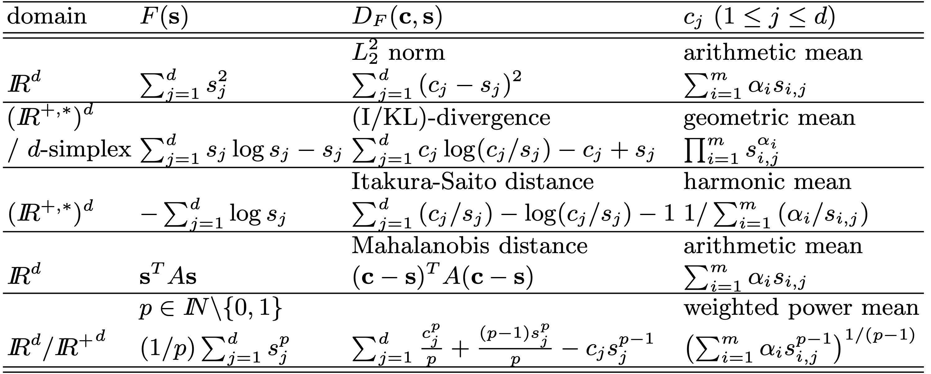Figure 2: Bregman divergences and their associated functional averages from (Nock and Nielsen, 2005). Some other divergences, not included in the above table, are the Hellinger distance and the linear-exponential (linex) loss, e.g., see Ackermann and Blömer (2009).

To clarify the notation in the table, we first note in the second and third column that $c$ is a vector and $s$ is an “arbitrary” vector, whereas in the fourth column, $s_i$ are given (i.e., data) vectors, where $1 \leq i \leq m$. The functional average in the fourth column could be seen as the minimizer of the “smallest enclosing” Bregman divergence with respect to the first argument. Ignoring the “smallest enclosing” constraint and setting $\alpha_i=1/m$, the $c$ in the last column is simply $\argmin_{c} \frac{1}{m} \sum_{i=1}^m D_F(c,s_i)$. The $\alpha_i$ are just Lagrange multipliers that come from the constrained problem: $\argmin_{r,c} \ r$, s.t. $D_F(c,s_i) \leq r$ for $1 \leq i \leq m$ (in the spirit of support vector machines). Namely, since $\frac{\partial}{\partial c} D_{F}(c,s_i) = \nabla F(c) - \nabla F(s_i)$, the functional average is $c^\ast = (\nabla F)^{-1}(\frac{1}{m} \sum_{i=1}^m \nabla F(s_i))$. Indeed, this is the arithmetic average when $F$ is the L2 norm as shown in the table.

There is also an interesting parallel in Bayesian decision making theory. When the risk of a classifier $\hat{y}$ is $R(\hat{y}) = \frac{1}{2} \E_{x,y} \|\hat{y}(x) - y\|^2$, then the Bayes optimal classifier is $\hat{y}_\text{Bayes}(x) = \E_{y|x}[y]$, which is like the arithmetic average. For L1 distance risk, we get the median instead of the average, but this is not necessarily the same for Bregman divergences. Remember that Bregman divergences are associated with differentiable and strictly convex functions (but see the last row in the table and take $p \to 1$, e.g.).

Mirror descent

Solving sub-problem $\eqref{eq:mirror-descent}$ gives the mirror descent step. First, note that $\nabla_x B_{\psi}(x,x_t) = \nabla \psi(x) - \nabla \psi(x_t)$. Then, taking the minimum by setting the gradient to 0 and rearranging, we get

\[\begin{equation*} \nabla \psi(x^{\text{opt}}) = \nabla \psi(x_t) - \eta_t \nabla f(x_t) \end{equation*}\]

which is a minimizer since $\psi$ is strictly convex. Recall that this gives preconditioned gradient descent when $\psi = \frac{1}{2}\|\cdot\|_D^2$ (which includes AdaGrad and Newton step).

It is called mirror descent because you’re sort of descending in the “mirror” world, aka the dual space. In other words, you go to the dual space, take a regular Euclidean gradient step there, and then come back. Namely,

\[\begin{equation} x_{t+1} = (\nabla \psi)^{-1}(\nabla \psi(x_t) - \eta_t \nabla f(x_t)), \end{equation}\]

where the inverse is element-wise. This is like a change of coordinates that makes the Euclidean metric “more natural”. For Euclidean space, the rate of change of the L2 norm is proportional to the variable itself, so no change of coordinates is required. On the other hand, for spaces with general norms of quadratic form $\|x\|_D^2=x^TDx$, we can linearly transform the coordinates $x'=D^{1/2}x$ so that the rate of change of the L2 norm of this parameterization is similar to the quadratic norm $\|x\|_D^2$ of this space. This intuition will help us understand BLR later.

Duality in mirror descent

We can explicitly solve the equation for $x$ by figuring out $(\nabla \psi)^{-1}$. In fact, $(\nabla \psi)^{-1} = \nabla \psi^\ast$, where $\psi^\ast$ is the convex conjugate of $\psi$. This is not clear at all, so let us see why it holds.

Recall the definition of the convex conjugate $\psi^\ast : \mathcal{X}^\ast \to \mathbb{R}$, where $\mathcal{X}^\ast$ is the dual space of $\mathcal{X}$

\[\begin{equation*} \psi^\ast(g) := \sup_{x} \langle g, x \rangle - \psi(x). \end{equation*}\]

Let’s take the supremum for each $\psi^\ast(g)$

\[\begin{equation*} \frac{\partial}{\partial x}\left(\langle g, x \rangle - \psi(x)\right) = 0 \quad\implies\quad g = \nabla \psi(x^{\text{opt}}). \end{equation*}\]

Note $x^{\text{opt}}$ is a maximizer since $-\psi(x)$ is strictly concave. Thus, for $x^{\text{opt}}$, the definition holds with equality $\psi^\ast(g) = \langle g, x^{\text{opt}} \rangle - \psi(x^{\text{opt}})$. By taking the gradient with respect to $g$, we get $\nabla \psi^\ast(g) = x^{\text{opt}}$. Thus,

\[\begin{equation*} g = \nabla\psi(\nabla\psi^\ast(g)) \quad \text{and} \quad x^{\text{opt}} = \nabla\psi^\ast(\nabla\psi(x^{\text{opt}})), \end{equation*}\]

which implies that $(\nabla\psi)^{-1} = \nabla\psi^\ast$.

This proof might not be rigorous, but it does the job. Even though the maximizer $x^{\text{opt}}$ kind of depends on $g$ (it’s right there in the definition of the convex conjugate), we did we not differentiate through it. I don’t know exactly why this works, but another intuitive way to look at it is through the subgradient (which becomes a gradient here because $x^{\text{opt}}$ is unique due to the strict convexity of $\psi$). Recall the definition of a subgradient $g$ of $\psi$ at $x$

\[\begin{equation*} g \in \partial\psi(x) \iff \psi(x') \geq \psi(x) + \langle g, x'-x \rangle, \ \forall x' \in \mathcal{X}. \end{equation*}\]

Let $x \in \mathcal{X}$ and $g \in \mathcal{X}^\ast$. Recall Fenchel-Young inequality (which directly follows from the definition of the convex conjugate)

\[\begin{equation*} \langle x, g \rangle \leq \psi(x) + \psi^\ast(g), \end{equation*}\]

which holds with equality when $g \in \partial\psi(x)$ (you can prove this key fact as an exercise). Using the biconjugate $\psi^{**}$, we also have

\[\begin{equation*} \langle x, g \rangle \leq \psi^{**}(x) + \psi^\ast(g), \end{equation*}\]

which similarly holds with equality when $x \in \partial\psi^\ast(g)$. Thus, since $\psi = \psi^{**}$ for lower semi-continuous $\psi$ (not gonna tell you why), we get

\[\begin{equation} g \in \partial\psi(x) \iff x \in \partial\psi^\ast(g). \label{eq:mirror-duality} \end{equation}\]

This is just the subgradient version of $(\nabla\psi)^{-1} = \nabla\psi^\ast$. For a rigorous treatment of the above, see Theorem 23.5 in Convex Analysis (Rockafellar, 1970).

Anyways, moving on.

Descending a valley as information

The previous analysis works when we have access to gradients or unbiased estimates thereof (i.e., stochastic gradients), and it assumes that we know the iterates exactly, which makes sense. However, we will see that we can also work with distributions over points instead, which is a powerful perspective that leads to inuitive understanding and derivation of optimization algorithms.

Reformulating the objective

Recall the original optimization objective

\[\begin{equation*} \argmin_{x} \quad f(x) + \Gamma(x), \end{equation*}\]

where $\Gamma$ is some regularizer, e.g., $\Gamma(x;\lambda) = \frac{\lambda}{2}\|x\|_2^2$.

We can change it slightly to allow for “errors” in $x$. We can either minimize with respect to the worst case or the expected case.

Let $\varepsilon$ be the perturbation or error variable. In the worst case scenario, we take the worst (i.e., maximizing) $\varepsilon$ under some constraint, e.g., $\|\varepsilon\|_p \leq r$ for some $p\geq 1$ and $r > 0$ (the constraint is needed as otherwise the max problem will be trivial). As for the expected case, we sample $\varepsilon$ from some distribution depending on our modeling assumptions, e.g., $\varepsilon \sim \mathcal{N}(0, \sigma^2 I_d)$. Thus, we can write the objectives as follows

\[\begin{align} &\argmin_{x}\ {\color{brown} \max_{\|\varepsilon\|_p \leq r}} \ f(x + \varepsilon) + \frac{\lambda}{2}\|x\|_2^2 \tag{SAM} \label{eq:sam} \\ &\argmin_{x}\ {\color{brown} \E_{\varepsilon \sim \mathcal{N}(0, \sigma^2 I_d)}} \ [f(x+\varepsilon)] + \frac{\lambda}{2}\|x\|_2^2 \tag{Bayes} \label{eq:bayes} . \end{align}\]

The first objective $\eqref{eq:sam}$ is exactly the ones studied in sharpness-aware minimization (Foret et al., 2020) (hence the acronym). The authors used a linear approximation in $\varepsilon$, which results in a closed form max. For example, for $p=2$, the maximum is $f\left(x+r\frac{\nabla f(x)}{\|\nabla f(x)\|_2}\right)$. The gradient is then taken at this perturbed point, i.e., $z_t = \frac{\nabla f(x)}{\|\nabla f(x)\|_2} \big{|}_{x = x_t}$ is fixed and taken as an adversarial noise so that $x_{t+1} \gets x_t - \eta_t \nabla f(x_t + r z_t)$.

What we are really interested in is the second objective, which looks similar to the first one. The name $\eqref{eq:bayes}$ comes from the use of expectation. It also comes from the fact that it can be interpreted as finding the maximum a posteriori estimator $\theta$ that has a prior $\mathcal{N}(0, \frac{1}{\lambda} I_d)$ and a posterior $\mathcal{N}(x, \sigma^2 I_d)$ in our case.

In fact, it has been shown recently that $\eqref{eq:bayes}$ is very much related to $\eqref{eq:sam}$. The answer is succinctly explained in the title of the paper: “SAM as an Optimal Relaxation of Bayes” (Möllenhoff and Khan, 2023). Namely, $\eqref{eq:sam}$ is an optimal relaxation of$\eqref{eq:bayes}$, where the relaxation is based on the convex biconjugate $f^{\ast\ast}$ and the word “optimal” comes from the fact that $f^{\ast\ast}$ is the optimal convex lower bound of $f$.

An information-theoretic objective

The $\eqref{eq:bayes}$ objective is more general as we can think in terms of posteriors $x \sim q_t$ rather than hard iterates $x_t$. Indeed, $\eqref{eq:bayes}$ can be written in terms of distributions using a variational formulation called the optimal information-processing rule $\eqref{eq:oipr}$, which is due to Zellner (1988, eq. 2.8)

\[\begin{equation} \argmin_q\ \E_{x \sim q} [f(x)] + D_{\text{KL}}(q(x)\, \|\, p(x) ), \tag{OIPR} \label{eq:oipr} \end{equation}\]

where $p$ is the prior of $x$, $q$ is the approximation of the posterior $p(x \mid \xi)$ given data $\xi$, and $D_{\text{KL}}$ is the KL-divergence, sort of like $\Gamma(x)$. Assuming a faithful negative log-likelihood (NLL) loss $f(x) \propto -\log p(\xi \mid x)$, the minimizer of $\eqref{eq:oipr}$ recovers the true posterior $p(x \mid \xi)$, which corresponds to Bayesian inference as a special case (see below).

Regarding notation, perhaps practitioners of Bayesian methods would be slightly confused, so let’s’ clarify things a bit. First, we are sticking with the optimization notation where $f$ is the loss, $x$ is the parameter of the model, not distribution (acting as the “latent” variable), and $\xi$ is the dataset (usually written in the literature as pairs of $x_i$ and $y_i$), which would be slightly irrelevant to BLR, at least in this post. Another source of confusion might be $D_{\text{KL}}(q(x)\, \|\, p(x) )$ as $q(x)$ should actually approach $p(x \mid \xi)$ as it gets better, not $p(x)$. The reason for that is a bit subtle and would be clear in the following derivation.

Let’s take a look at the evidence lower bound (ELBO), which I will not discuss in details as it warrants an article on its own, but let’s assume that it’s given.

\[\begin{align} \mathcal{L}(q) &:= \E_{x \sim q}\left[ \log \frac{p(x,\xi)}{q(x)} \right] \tag{ELBO} \label{eq:elbo} \\ &= \underbrace{\log p(\xi)}_{\text{evidence}} - \underbrace{D_{\text{KL}}(q(x)\, \|\, p(x|\xi) )}_{\geq 0} \leq \log p(\xi). \nonumber \end{align}\]

Maximizing the ELBO implies a better lower bound for the evidence. Cool, so how is this related to $\eqref{eq:oipr}$? It’s straightforward, actually. Just plug in the negative log-likelihood loss

\[\begin{align*} \text{(OIPR)'s obj.} &= \E_{x \sim q} \left[\log \frac{q(x)}{p(\xi|x)p(x)}\right] + \text{const} \\&= \E_{x \sim q} \left[\log \frac{q(x)}{p(x|\xi)p(\xi)}\right]+ \text{const} \\&= -\text{(ELBO)} + \text{const}, \end{align*}\]

so that minimizing $\eqref{eq:oipr}$’s objective given $f(x) \propto -\log p(\xi \mid x)$ implies maximizing the ELBO, as shown in (Khan & Rue, 2023, p. 28)².

Beyond “point” gradients

We now come to the crux of this blog post. Can we solve $\eqref{eq:oipr}$ with gradient descent? What does it mean to take a gradient descent step on $q$? Does $q_{t+1} = q_t - \eta_t \nabla_q \left(\E_{x \sim q} [f(x)] + D_{\text{KL}}(q(x)\, \|\, p(x) ) \right)$ make sense? Yes, kind of! Not only does it make sense, we should sometimes think of it this way. Let’s see why next.

Descending like a Bayesian

Generally speaking, posteriors are positive functions that integrate to 1. A perturbed posterior $\tilde{q}$ can be controlled in terms of norms, e.g. $\|\tilde{q}-q\|_1 < \epsilon$. But it is intractable to “describe” such functions for every possible sample $x \in \mathcal{X}$, let alone perturb them (i.e., as in lookup tables).

The common way to describe and control probability distributions is by parameterizing³ them under some constraints and assumptions. This way, instead of working with functions, we work with their parameters instead as they are fully described by them. In general, the constraints and assumptions (including parameterization) describe the distribution family, and the parameter choice describes a member of the family (and not a sample).

Quite often, this parameter space is not Euclidean, i.e., the parameter entries do not vary at the same rate with respect to each other. For example, for the normal/Gaussian posterior family, the mean and covariance are the natural parameters that fully characterize a normal posterior. Perturbing the mean of the distribution changes the samples in a completely different manner than perturbing the covariance. The mean shifts the position, while the variance controls the deviation/scattering. It is, thus, obvious that the position and the deviation do not vary at the same rate.

We will see next that solving $\eqref{eq:oipr}$ with posteriors from the exponential family of distributions⁴ corresponds to preconditioned gradient descent with an exponentially smoothed Hessian as a preconditioner.

Side-quest: minimizing perturbations around the mean

An interesting thing happens, for example, when we minimize the second-order taylor expansion of the functional $F(q) := \E_{x \sim q} [f(x)]$ around the mean $\mu := \E_{x \sim q} [x]$ (let’s ignore the KL divergence term for now)

\[\begin{equation*} F(q) \approx f(\mu) + \underbrace{\E_{x \sim q} (x - \mu)^T\nabla f(\mu)}_{=0} + {\small \frac{1}{2}}\E_{x \sim q} (x - \mu)^T\nabla^2 f(\mu) (x - \mu). \end{equation*}\]

Observe that the first-order expansion simply recovers the regular objective with respect to hard iterates. Let $\Sigma := \E_{x \sim q} [(x-\mu)(x-\mu)^T]$ be the covariance of $x$, which is symmetric. Then,

\[\begin{align*} F(q) &\approx f(\mu) + {\small \frac{1}{2}}\E_{x \sim q} \text{Tr}((x - \mu)^T \nabla^2 f(\mu) (x - \mu)) \\ &= f(\mu) + {\small \frac{1}{2}}\E_{x \sim q} \text{Tr}((x - \mu)(x - \mu)^T \nabla^2 f(\mu)) \\ &= f(\mu) + {\small \frac{1}{2}}\text{Tr}(\Sigma \nabla^2 f(\mu)). \end{align*}\]

The expression $\text{Tr}(\Sigma \nabla^2 f(\mu))$ can also be written $\langle \Sigma , \nabla^2 f(\mu) \rangle_\text{F}$, which is the Frobenius inner product.

Thus, approximating the objective $\argmin_q F(q)$ given the mean and the covariance of $q$ gives

\[\begin{equation} \argmin_{q} \ \E_{x \sim q} [f(x)] \approx \argmin_{\mu, \ \Sigma} \ f(\mu) + {\small \frac{1}{2}} \langle \Sigma , \nabla^2 f(\mu) \rangle_\text{F}. \end{equation}\]

Thus, we cast the problem of minimizing the Bayesian objective with respect to posteriors $q$ to a more tractable problem in terms of the mean and covariance of $q$ only, which is accurate up to second-order terms. Note that we have not made any assumptions about $q$ other than that its mean and covariance exist.

Interestingly, if we fix $\Sigma = I$, the Bayesian objective implicitly flattens the minimizer via a Hessian sharpness penalty, i.e., $\langle \Sigma , \nabla^2 f(\mu) \rangle_\text{F} = \text{Tr}(\nabla^2 f(\mu))$. In some sense, $\Sigma$ can be seen as a preconditioner (more details on this later). Therefore, optimizing the second-order approximation of $\eqref{eq:oipr}$’s objective by tuning the preconditioner $\Sigma$ might yield lower objective values than a fixed preconditioner (as in $\Sigma = I$), but this can happen at the expense of a sharper Euclidean minimum when $f$ is non-convex. Perhaps running Adam with a preconditioner that decays to $\frac{1}{\eta_t}I$ can converge to a solution that generalizes better. Pretty sure this was already investigated in the literature, but I’m too lazy to look it up now.

The Bayesian Learning Rule (BLR)

We now derive a gradient descent update for $\eqref{eq:oipr}$. Let the parameter of posterior $q$ be $\theta \in \mathbb{R}^D$ for some $D$ (recall that $d$ is the dimension of the model sampled from this posterior). The posterior is denoted as $q_\theta(x)$, which we will try to maintain explicitly for clarity.

Note: I’m using $\theta$ to denote the natural parameter and $x$ a sampled model from $q_\theta$, which is quite different from the BLR paper, so I’m sorry about the confusing notation, but this one feels more natural to my eyes.

The exponential family of distributions

The first component of the Bayesian Learning Rule (Khan and Rue, 2023) is the assumption that $q_\theta(x)$ is an exponential-family (EF) distribution. Namely,

\[\begin{equation} q_\theta (x) = h(x) \exp \left( \langle \theta, T(x) \rangle - A(\theta) \right). \tag{EF} \label{eq:ef} \end{equation}\]

The variable $\theta$ is called the natural parameter (e.g., $\theta = [\mu; \vec(\Sigma)] \in \mathbb{R}^{D+D^2}$ for normal distributions⁵), and $A(\theta)$ is the log-partition function $\log \int h(x) e ^{ \langle \theta, T(x) \rangle} dx$, which normalizes the probability $q_\theta (x)$. The function $h(x)$ is the base measure, i.e., $q_{0}(x) \propto h(x)$. In a measure theoretic formulation, we can write $dq_{\theta}(x) = e ^{ \langle \theta, T(x) \rangle - A(\theta)} dh(x)$. Since we are interested in maximizing $\log q_\theta (x)$ over $\theta$, we can simply ignore $h(x)$. Finally, $T(x)$ is the sufficient statistic, and we can see that the log-probability is proportional to $\langle \theta, T(x) \rangle$, so we only need $T(x)$ from $x$ in order to calculate $q_{\theta}(x)$.

EF distributions can be written in other forms as well, but the one we show here is the one that “makes sense” when we want to maximize $\log q_{\theta}(x)$. Maximizing $\log q_{\theta}(x)$ by setting its gradient to zero amounts to finding $\theta$ such that $T(x) = \nabla A(\theta)$. Since $A(\theta)$ is strongly convex and differentiable, its gradient is invertible, so we have $\theta^\text{opt} = (\nabla A)^{-1}(T(x))$. But looking more carefully at $\max_{\theta} \log q_{\theta}(x)$, it is just $\sup_{\theta} \langle \theta, T(x) \rangle - A(\theta) = \langle \theta^\text{opt}, T(x) \rangle - A(\theta^\text{opt})$. This is precisely the definition of $A^\ast(T(x))$, from which we have $\theta^\text{opt} = \nabla A^\ast(T(x))$. Oh wait, we have seen something like this before! Looking back at the mirror descent section, we can see why it holds that

\[\begin{equation*} \theta^\text{opt} = (\nabla A)^{-1}(T(x)) = \nabla A^\ast(T(x)). \end{equation*}\]

Indeed, this is one of the main perks of EF distributions. More on this below.

The BLR update

The second component of the Bayesian Learning Rule is the BLR step, which is a natural gradient descent step for $\eqref{eq:oipr}$ (with respect to the natural parameter)

\[\begin{equation} \theta_{t+1} = \theta_{t} - \eta_t \tilde{\nabla}_{ {\color{brown}\theta_t}} f_{\text{OIPR}}(q_{ {\color{brown}\theta_t}}), \tag{OIPR-step} \label{eq:oipr-step} \end{equation}\]

where $f_{\text{OIPR}}(q) = \E_{x \sim q} [f(x)] + D_{\text{KL}}(q(x)\, \|\, p(x) )$ and $\tilde{\nabla}$ is the natural gradient.

By assuming a regularizer $\Gamma(x) = - \log p(x)$ and noting that $D_{\text{KL}}(q(x)\, \|\, p(x) ) = \E_{x \sim q} [\Gamma(x)] - H(q)$, where $H(q) = -\E_{x \sim q}[\log q(x)]$ is the entropy, the BLR paper writes $\eqref{eq:oipr-step}$ in terms of the loss $f$, the regularizer $\Gamma$, and the entropy $H$ as

\[\begin{equation} \theta_{t+1} = \theta_{t} - \eta_t \tilde{\nabla}_{ {\color{brown}\theta_t}} (\E_{x \sim q_{ {\color{brown}\theta_t}} } [f(x) + \Gamma(x)] - H(q_{ {\color{brown}\theta_t}})). \tag{BLR-step} \label{eq:blr-step} \end{equation}\]

Recall that for a NLL loss, i.e., $f(x) \propto - \log p(\xi \mid x)$, solving $\eqref{eq:oipr}$ is equivalent to maximizing $\eqref{eq:elbo}$, and the optimal solution is $q^\ast = p(\cdot \mid \xi)$.

Natural gradient

The elegant mechanism that ties $\eqref{eq:ef}$ and $\eqref{eq:blr-step}$ together and take them to the next level is the natural gradient $\tilde{\nabla}$. The natural gradient uses the inverse Fisher information matrix $\fisher(\theta)$ as a preconditioner for the gradient

\[\begin{equation} \tilde{\nabla}_{\theta} \E_{x \sim q_{\theta}}(\cdot) = \fisher(\theta)^{-1} \nabla_{\theta} \E_{x \sim q_{\theta}} (\cdot). \tag{NG} \label{eq:ng} \end{equation}\]

What is the fisher information matrix (FIM)? The most straightforward description is that the FIM measures the expected (observed) information that samples $x \sim q_{\theta}$ have about $\theta$. Technically speaking, $\fisher(\theta)$ is the covariance of the score $\nabla_\theta \log q_\theta(x)$. Namely,

\[\begin{equation} \fisher(\theta) = \E_{x \sim q_{\theta_t}} [\nabla_\theta \log q_\theta(x) \nabla_\theta^T \log q_\theta(x)] = \E_{x \sim q_{\theta_t}} [-\nabla_\theta^2 \log q_\theta(x)] , \tag{FIM} \end{equation}\]

which is a covariance since $\E_{x \sim q_{\theta_t}} [\nabla_\theta \log q_\theta(x)] = 0$ (as long as the regularity conditions for $\int \nabla_\theta = \nabla_\theta \int$ hold). The third identity can be shown to be equal to the second by solving it directly (this time, using $\int \nabla_\theta^2 = \nabla_\theta^2 \int$). Recalling the expression of $q_{\theta}(x)$, it is then easy to see that

\[\begin{equation} \fisher(\theta) = \nabla_{\theta}^2 A(\theta). \tag{EF-FIM} \end{equation}\]

This is interesting because we can already see that some kind of a Newton step is happening. We will see the implications of this identity as we move on.

Expectation parameters and duality

Using the fact that the expectation of the score is 0, we immediately see, again from the expression of $q_{\theta}(x)$, that

\[\begin{equation} \nabla A(\theta) = \E_{x \sim q_{\theta}}[T(x)] =: \nu(\theta) \tag{Expect. param.} , \end{equation}\]

which is the definition of the expectation parameter $\nu$. It is very similar to the condition of the maximizer $\theta^{\text{opt}}$ for $\log q_\theta (x)$, but here, we have the sufficient statistic in expectation, which is an important distinction. Note that the equality above holds for all $\theta$ due to the fact that the expectation of the score is 0 for all $\theta$.

The astute reader should now be able to see the duality between $\theta$ and $\nu$. The definition of the expectation parameter and the discussion in the mirror descent section already hint at this duality. Indeed, we have

\[\begin{equation} \nu = \nabla A(\theta) , \quad\quad \theta = \nabla A^\ast(\nu) . \tag{BLR duality} \end{equation}\]

We dropped the dependence of $\nu$ on $\theta$ here on purpose because $\theta$ depends on $\nu$, too! This is exactly the same story when we showed $\nabla \psi^\ast = (\nabla \psi)^{-1}$ in mirror descent. The parameters $\theta$ and $\nu$ exist in dual worlds and are coupled by $A$ as much as $x$ and $g$ are coupled by $\psi$.

Given this duality, the following elegant formula of the natural gradient can be derived with some derivative shenanigans

\[\begin{equation} \tilde{\nabla}_{\theta} \E_{x \sim q_{\theta}}(\cdot) = \nabla_{\nu} \E_{x \sim q_{\theta}} (\cdot) . \end{equation}\]

It follows mainly from the fact $\nabla_\theta \nu = \nabla^2 A(\theta) = \fisher(\theta)$. Focusing solely on the derivative operator, we can derive it easily as follows

\[\begin{equation*} \tilde{\nabla}_{\theta} = \fisher(\theta)^{-1} \nabla_{\theta} = \left( \frac{\partial \nu}{\partial \theta} \right)^{-1} \frac{\partial}{\partial \theta} = \frac{\partial}{\partial \nu} = \nabla_{\nu} . \end{equation*}\]

Informally, we can say that the natural gradient in $\theta$ space is equal to the Euclidean gradient in $\nu$ space.

Why natural gradients?

Is the choice of the natural gradient just a matter of convenience? Not really. At least not when $q$ is an EF distribution.

One important property of natural gradient descent is that it is invariant to reparameterizations of $\theta$, so it depends directly on $q_\theta$. This is one of the main ideas behind information geometry. It doesn’t matter whether you use the standard deviation or the variance in $\theta$. Natural gradient descent will yield the same iterates, so it is a proper gradient descent on $q$ that acts on the (parameterized) distribution rather than the natural parameter itself.

Another interesting reason stems from the gradient of the entropy in $\eqref{eq:blr-step}$. Let $F(q) := \E_{x \sim q } [f(x) + \Gamma(x)]$ and consider a fixed point $\theta^\text{opt}$ of $\eqref{eq:blr-step}$ so that

\[\begin{equation*} 0 = \tilde{\nabla}_{\theta} (F(q_{\theta^\text{opt}}) - H(q_{\theta^\text{opt}})). \end{equation*}\]

Assuming that the base measure $h(x)$ is constant, we can show that the natural gradient of the negative entropy $-H(q_\theta)$ is simply $\theta$, whereas the Euclidean gradient is $\nabla^2 A(\theta) \theta$ (see the appendix for the full details). This implies the following identity of the fixed point

\[\begin{equation*} \theta^\text{opt} = -\tilde{\nabla}_{\theta} F(q_{\theta^\text{opt}}). \end{equation*}\]

Even if we use the Euclidean gradient in $\eqref{eq:blr-step}$, we would have

\[\begin{equation*} \nabla^2 A(\theta^\text{opt}) \theta^\text{opt} = -\nabla_{\theta} F(q_{\theta^\text{opt}}), \end{equation*}\]

which immediately implies the previous identity since $\fisher(\theta) = \nabla^2 A(\theta^\ast)$. This suggests that the natural gradient is inherent in every solution of $\eqref{eq:oipr}$.

There is a simple interpretation behind this phenomenon. Consider a regularized problem $f(x) + \frac{1}{2}\|x\|_D^2$ for some $D \succ 0$. The optimal $x^\text{opt}$ is characterized by the identity $Dx^\text{opt} = -\nabla f(x^\text{opt})$, so we can similarly argue that the preconditioned gradient $D^{-1} \nabla f(x)$ is inherent in every solution. However, this is particularly because $D$ is the underlying metric in the regularizer. For $\eqref{eq:oipr}$ with EF distributions, the metric induced by the entropy is $\fisher(\theta) = \nabla^2 A(\theta)$.

Note that the Euclidean gradient of the negative entropy $-H(q_{\theta})$ is a (invertible) linear transformation of $\theta$. The negative entropy is strictly convex in $q$, so with some manipulations (as per the mirror descent section above), we can get $(\nabla H)^{-1}(-q^*) = \nabla (-H)^\ast(q^*)$ for some arbitrary dual variable $q^*$. Thus, we can obtain the following generalized expression

\[\begin{equation} \theta^\text{opt} = \nabla (-H)^\ast(\tilde{\nabla}_\theta F(q_{\theta^\text{opt}})), \end{equation}\]

Indeed, this can be understood as mirror descent on distributions with $-H$ as the potential, which induces the metric via the Bregman divergence (i.e., the KL-divergence). This gives an intuition on the correspondence between potentials and entropies (resp., divergences and metrics). We will make this correspondence more concrete in the next section.

Natural gradient descent and mirror descent

The BLR step $\eqref{eq:blr-step}$ is intimately related to mirror descent, and mirror descent is just gradient descent in the dual space, i.e., the space where the metric is Euclidean.

Natural gradient descent, as mirror descent, obtains the descent step from minimizing a sub-problem involving an approximation of the objective. Ignoring the constant terms, the natural gradient descent sub-problem is

\[\begin{equation} \theta_{t+1} \gets \argmin_{ {\color{brown} \theta}} \ \langle \nabla_\theta f(q_{\theta_t}), {\color{brown} \theta} \rangle + \frac{1}{\eta_t} D_\text{KL} (q_{ {\color{brown} \theta}} \| q_{\theta_t}). \end{equation}\]

The minimization of the KL-divergence (or any f-divergence) can be made easy with some second-order approximation magic (you can find a derivation here under the “Proximal-gradient descent” section, for example)

\[\begin{equation*} D_\text{KL} (q_{ {\color{brown} \theta}} \| q_{\theta_t}) \approx ({\color{brown} \theta} - \theta_t)^T \fisher(\theta_t) ({\color{brown} \theta} - \theta_t). \end{equation*}\]

Using this approximation, we obtain

\[\begin{equation} \theta_{t+1} \gets \theta_t - \eta_t \fisher(\theta_t)^{-1}\nabla_\theta f(q_{\theta_t}), \end{equation}\]

which is the natural gradient descent step.

We can derive the same update with mirror descent assuming that $q_\theta$ is an EF distribution. In this case, mirror descent is exactly natural gradient descent because the second-order approximation of the KL-divergence is exact for EF distributions. However, natural gradient descent is not always equivalent to mirror descent. This distinction happens mainly when the natural parameter space is constrained or when the second-order taylor expansion of the KL-divergence is not exact (for details, see this).

Now let’s see how the natural gradient descent can be derived from mirror descent for EF distributions. Recalling the duality $\nu(\theta) = \nabla A(\theta)$ and $\theta = \nabla A^*(\nu)$ (where we sometimes write $\nu$ as a function of $\theta$ for clarity), the KL-divergence can conveniently be rewritten as follows

\[\begin{align*} D_\text{KL} (q_{ {\color{brown} \theta}} \| q_{\theta_t}) &= \E_{x \sim q_{ {\color{brown} \theta}}} [\log q_{ {\color{brown} \theta}}(x)] - \E_{x \sim q_{ {\color{brown} \theta}}} [\log q_{\theta_t}(x)] \\ &= \langle {\color{brown} \theta}, \nu({\color{brown} \theta}) \rangle - A({\color{brown} \theta}) - \langle \theta_t, \nu({\color{brown} \theta}) \rangle + A(\theta_t) \\ &= A(\theta_t) - A({\color{brown} \theta}) - \langle \theta_t - {\color{brown} \theta}, \nabla A({\color{brown} \theta}) \rangle \\ &= B_{A} (\theta_t, {\color{brown} \theta}), \end{align*}\]

which is the Bregman divergence corresponding to $A$. The divergence term is also equal to the reverse divergence in the dual space, i.e., $B_{A} (\theta_t, {\color{brown} \theta}) = B_{A^\ast} (\nu({\color{brown} \theta}) , \nu(\theta_t))$. The derivation is straightforward and can be found in the appendix.

This equality implies that we can write the natural gradient descent sub-problem in terms of mirror descent with respect to $\nu({\color{brown} \theta})$ given a reparameterized loss $\tilde{f}(\nu(\theta_t)) = f(q_{\theta_t})$ as follows

\[\begin{equation} \nu_{t+1} \gets \argmin_{ {\color{brown}\nu}} \ \langle \nabla \tilde{f}(\nu_t), {\color{brown}\nu} \rangle + \frac{1}{\eta_t} B_{A^\ast} ({\color{brown} \nu } , \nu_t) . \end{equation}\]

Indeed, $\nabla_{ {\color{brown} \nu }} B_{A^\ast} ({\color{brown} \nu } , \nu_t) = {\color{brown} \nu } - \nu_t$ and $\nabla_\nu \tilde{f} = F^{-1} \nabla_\theta f$. This shows the equivalence between mirror descent and natural gradient descent for EF distributions.

BLR steps in the wild

Ok, so the most important question is: How do we get something practical out of BLR?

By now, the keen eye will notice that some kind of a preconditioned gradient descent should follow from BLR. Preconditioned gradient descent already covers a large number of algorithms, including Newton and AdaGrad, for example. The versatility of BLR in deriving different practical algorithms is surprising given the simplicity and universality of its assumptions (EF distributions and natural gradients) and the theory-driven derivations, which leads to principled algorithmic practices that are often experiment and engineering-driven.

In this section, we will derive the Newton method from BLR, but before that, we will go through preliminaries about sufficient statistics and the delta method, which can be safely skipped if the reader already knows enough about them.

From now on, we will set $\Gamma(\cdot)=0$ for simplicity, as this choice is orthogonal to the derivation of the algorithms. Alternatively, the reader can think of $\Gamma$ as being already built into $f$.

Sufficient statistic

An important concept that we have introduced without much explanation is the sufficient statistic.

We implicitly defined the sufficient statistic by its presence in the expression of EF distributions $q_\theta(x) = h(x) \exp (\langle \theta, T(x) \rangle - A(\theta))$. Given $\theta$, the distribution over $x$ is completely determined by its statistic $T(x)$ (up to normalization). In other words, knowing $T(x)$ about $x$ is sufficient to estimate $\theta$ exactly, and knowing more than $T(x)$ is not necessary. (Note this does not mean that knowing $T(x)$ is necessary, in which case it would be called the minimal sufficient statistic.)

Sufficient statistics go beyond EF distributions (in a straightforward manner). The Fisher–Neyman factorization theorem says that, in general, we have $q_\theta(x) = h(x) g_\theta(T(x))$ for non-negative $h$ and $g_\theta$. The EF case is when $g_\theta$ is a linear function. Furthermore, sufficient statistics can be transformed by bijections and still maintain their sufficiency. This is simply because we can always invert bijections.

Let’s see some examples. A sufficient statistic for normal distirbutions is $T(x) = [\hat{\mu}(x); \hat{\sigma}(x)^2]$, where $\hat{\mu}(x) = \frac{1}{n} \sum_i x_i$ and $\hat{\sigma}(x)^2 = \frac{1}{n-1} \sum_i (x_i - \hat{\mu}(x))^2$. Multiplication by a constant still maintains the sufficiency because all the information is “already there” and we just need to rescale it to correct for bias. In fact, $T(x)=\sum_i x_i$ is a sufficient statistic for both Poisson distributions and exponential distributions. Observe that both of them are EF distributions, as is the normal distribution, so it should be clear why the scale does not remove the sufficiency. As another intuitive example, a sufficient statistic for estimating the uniform distribution $\mathcal{U}(0, \theta)$ from samples $x = (x_1, \cdots, x_n)$ is $T(x) = \max_{1 \leq i \leq n} x_i$.

Delta method

One common trick for deriving practical algorithms is the delta method. We have already used a better version of it before. The delta method is simply a first-order approximation around the mean, so what you will get is just the function itself evaluated at the mean. Namely, for $\mu := \E_{x \sim q_\theta}[x]$, we get

\[\begin{equation} \E_{x \sim q_\theta}[f(x)] \approx \E_{x \sim q_\theta}[f(\mu) + \langle \nabla f(\mu), x - \mu \rangle] = f(\mu). \tag{Delta-0} \end{equation}\]

I kinda hate it because it is a crude approximation that ignores the variance. For example, imagine you have a normally distributed $q_\theta$ with $\mu=0$. This approximation simply says that $\E_{x \sim q_\theta}[f(x)] = f(0)$. This is an optimistic approximation and it does make sense, but consider the second order approximation $f(0) + \frac{1}{2} \langle \Sigma, \nabla^2 f(0) \rangle_{\text{F}}$, where $\Sigma = \E_{x \sim q_\theta}[xx^T]$. If $\Sigma^{-1} = \nabla^2 f(0)$, the second-order term is constant. Otherwise, the dependence of $\theta$ on the second-order term can be non-trivial. Therefore, the first-order approximation is bad particularly when the curvature of $f$ is ill-shaped with respect to $\Sigma^{-1}$.

An extension of the delta method to gradients and Hessians of $f$ is possible as well and is very useful. For gradients, we use Bonnet’s Theorem (Bonnet, 1964)

\[\begin{equation} \E_{x \sim q_\theta}[\nabla f(x)] = \nabla_{\mu} \E_{x \sim q_\theta}[f(x)]. \tag{Bonnet} \end{equation}\]

This is only helpful if we can write the inner part in terms of $\mu$, but we can use the delta method to have

\[\begin{equation} \E_{x \sim q_\theta}[\nabla f(x)] \overset{(\text{Bonnet})}{=} \nabla_{\mu} \E_{x \sim q_\theta}[f(x)] \approx \nabla f(\mu). \tag{Delta-1} \label{eq:delta-1} \end{equation}\]

As for the Hessian, we use Price’s Theorem (Price, 1958)

\[\begin{equation} \E_{x \sim q_\theta}[\nabla^2 f(x)] = 2 \nabla_{\Sigma} \E_{x \sim q_\theta}[f(x)]. \tag{Price} \end{equation}\]

This time, we use a second-order approximation $f(\mu) + \frac{1}{2} \langle \Sigma, \nabla^2 f(\mu) \rangle_{\text{F}}$ to get

\[\begin{equation} \E_{x \sim q_\theta}[\nabla^2 f(x)] \overset{(\text{Price})}{=} 2 \nabla_{\Sigma} \E_{x \sim q_\theta}[f(x)] \approx \nabla^2 f(\mu). \tag{Delta-2} \label{eq:delta-2} \end{equation}\]

Deriving Newton’s Method from BLR

Now we have the necessary tools to proceed. Instead of deriving gradient descent from BLR, we will jump straight to Newton’s method, from which it will be easy to see how vanilla gradient descent can be derived.

The main assumption we use here is that $q_{\theta}$ is a normal distribution, with natural parameter $\theta = [\theta^{(1)}; \theta^{(2)}]$ and

\[\begin{align*} \theta^{(1)} &= \Sigma^{-1} \mu, \\ \theta^{(2)} &= - \frac{1}{2} \Sigma^{-1}. \end{align*}\]

We didn’t come up with this parameterization. This is the natural parameter of a (multi-variate) normal distribution obtained from writing its distribution as $h(x) \exp (\langle T(x), \theta \rangle - A(\theta))$.

On the other hand, the expectation parameter $\nu(\theta)$ depends on the choice of $T(x)$. Using the straightforward sufficient statistic $T(x) = [x; xx^T]$, we obtain

\[\begin{align*} \nu^{(1)} &= \mu , \\ \nu^{(2)} &= \Sigma + \mu\mu^T , \end{align*}\]

where the second equality follows because $\E[(x-\mu)(x-\mu)^T] = \E[xx^T] - \mu\mu^T$. Note again that $\nu$ depends on $T(x)$ and not on $\theta$.

Now recall that $-\nabla H(q_{\theta_t}) = \theta_t$ for constant base measures $h(x)$ (see the appendix), which is the case for normal distributions. Thus, $\eqref{eq:blr-step}$ becomes

\[\begin{align} \theta_{t+1} &= \theta_{t} - \eta_t \tilde{\nabla}_\theta \E_{x \sim q_{\theta_t}} [f(x)] + \eta_t \tilde{\nabla}_\theta H(q_{\theta_t}) \nonumber \\ &= (1-\eta_t) \theta_{t} - \eta_t \nabla_\nu \E_{x \sim q_{ {\theta_t}} } [f(x)]. \label{eq:gaussian-blr-step} \end{align}\]

What remains to figure out is $\tilde{\nabla}_{ {\theta_t}} \E_{x \sim q_{ {\theta_t}} } [f(x)]$.

Remember the chain rule trick we did that says $\tilde{\nabla}_{ {\theta_t}} = \nabla_{ \nu_t}$? Great, but now we have two partitions that are not necessarily independent, i.e., with respect to our practical parameterization, namely $\tilde{\theta} = [\mu; \text{vec}(\Sigma)]$. In practice, we optimize with respect to $\tilde{\theta}$, so we should write $\eqref{eq:blr-step}$ in terms of $\mu$ and $\Sigma$.

Let’s figure out the gradients $\nabla_{\nu^{(1)}}$ and $\nabla_{\nu^{(2)}}$ first. Let $h(\mu, \Sigma)$ be an arbitrary differentiable function, acting as a reparameterized proxy of $\E_{x \sim q_{\theta} } [f(x)]$.

From the expression of $\nu$, we can write $\Sigma = \nu^{(2)} - \nu^{(1)} (\nu^{(1)})^T$, so

\[\begin{equation*} \frac{\partial h}{\partial \nu^{(1)}} = \frac{\partial h}{\partial \mu} \frac{\partial \mu}{\partial \nu^{(1)}} + \frac{\partial h}{\partial \Sigma} \frac{\partial \Sigma}{\partial \nu^{(1)}} = \frac{\partial h}{\partial \mu} - 2 \frac{\partial h}{\partial \Sigma} \mu, \end{equation*}\]

and

\[\begin{equation*} \frac{\partial h}{\partial \nu^{(2)}} = \frac{\partial h}{\partial \Sigma} \frac{\partial \Sigma}{\partial \nu^{(2)}} = \frac{\partial h}{\partial \Sigma}. \end{equation*}\]

In other words,

\[\begin{equation} \begin{aligned} \nabla_{\nu^{(1)}}h(\cdot) &= \nabla_\mu h(\cdot) - 2 \nabla_{\Sigma}h(\cdot) \mu, \\ \nabla_{\nu^{(2)}}h(\cdot) &= \nabla_{\Sigma} h(\cdot) . \end{aligned} \label{eq:gaussian-nu-grad} \end{equation}\]

Let $h(\mu,\Sigma) =\E_{x \sim q_{\theta} } [f(x)]$ and plug in the gradients into $\eqref{eq:gaussian-blr-step}$, and then invoke $\eqref{eq:delta-1}$ and $\eqref{eq:delta-2}$ to get

\[\begin{align} \theta_{t+1}^{(1)} &= (1-\eta_t)\theta_{t}^{(1)} - \eta_t \nabla_\mu \E_{x \sim q_{\theta_t}} [f(x)] + 2\eta_t \nabla_\Sigma \E_{x \sim q_{\theta_t}} [f(x)] \mu_t \nonumber \\ &= (1-\eta_t)\theta_{t}^{(1)} - \eta_t \nabla f(\mu_t) + \eta_t \nabla^2 f(\mu_t)\mu_t , \\ \theta_{t+1}^{(2)} &= (1-\eta_t)\theta_{t}^{(2)} - \eta_t \nabla_\Sigma \E_{x \sim q_{\theta_t}} [f(x)] \nonumber \\ &= (1-\eta_t)\theta_{t}^{(2)} - \frac{\eta_t}{2} \nabla^2 f(\mu_t) . \end{align}\]

Writing the natural parameters $\theta_{t+1}^{(1)}$ and $\theta_{t+1}^{(2)}$ with respect to $\mu$ and $\Sigma$, we get

\[\begin{align} \Sigma_{t+1}^{-1} &= (1-\eta_t)\Sigma_{t}^{-1} + \eta_t \nabla^2 f(\mu_t) \\ \mu_{t+1} &= \Sigma_{t+1}\left[ {\color{brown} (1-\eta_t) \Sigma_{t}^{-1}} \mu_{t} - \eta_t \nabla f(\mu_t) + {\color{brown} \eta_t \nabla^2 f(\mu_t)} \mu_t) \right] \nonumber \\ &= \Sigma_{t+1}\left[ \Sigma_{t+1}^{-1}\mu_{t} - \eta_t \nabla f(\mu_t) \right] \nonumber \\ &= \mu_{t} - \eta_t \Sigma_{t+1} \nabla f(\mu_t) . \end{align}\]

It’s amazing how the covariance conveniently factored out and gave us Newton’s update. Not only did we get Newton’s method, but we also got an exponentially smoothed Hessian naturally from the theory for free.

It is straightforward to see how other algorithms can be derived from this one. For example, gradient descent is a special case when $\Sigma = I$. AdaGrad is a special case when we ignore the entropy of $\Sigma$ and approximate the covariance with the inverse of $\nabla f(\mu_t) \nabla^T f(\mu_t)$. Adam without momentum (i.e., $\beta_1=0$) is a special case when we use a similar approximation of the covariance but take the diagonal only (and we don’t ignore the entropy of $\Sigma$ here to keep the exponential smoothing). Dropout can also be explained with BLR (Khan and Rue, 2023, Sec. 4.3), which we will touch upon later.

The only interesting and very useful part of practical algorithms that BLR did not cover is momentum. It is possible to derive momentum from BLR given an adjusted sub-problem involving an extra divergence term from the previous iterate (see the paper). Perhaps a derivation of momentum is possible through a smart choice of $q_{\theta}$, but I’m not aware of it.

Side-quest: covariance approximation with stochastic gradients

In practice, we actually estimate the gradient of the minibatch $g=\frac{1}{B} \sum_{i=1}^B \nabla f(\mu_t; \xi_i)$ and then use $\sqrt{g \circ g} + \epsilon$ as the preconditioner. The square root is often taken for granted, but if you look closely, there is a subtle difference between how we approximate the Hessian and what we use as the preconditioner. Namely, $\sqrt{g \circ g} = \frac{1}{B} \sqrt{\sum_{i=1}^B \nabla f(\mu_t; \xi_i) \circ \sum_{i=1}^B \nabla f(\mu_t; \xi_i)}$, whereas the actual (unbiased) approximation should be something like $\frac{1}{B}\sum_{i=1}^B \sqrt{\nabla f(\mu_t; \xi_i) \circ \nabla f(\mu_t; \xi_i)}$. This is discussed in more details in Lin et al. (2024).

Specialized BLR steps in the wild

The multi-variate normal distribution is the most standard EF distribution, but EF distributions come in other flavors as well. Can we derive specialized algorithms for more specialized distributions? Yeah, why not.

Bernoulli (aka binary weights)

Binary weights (e.g., -1 and +1 weights) are difficult to train without making some simplifications. In practice, a straight through estimator (Bengio et al., 2013) is often used for the gradients. The straight through estimator is simple; we take a normal gradient descent step by pretending the weights are continuous but happen to be have discrete values, and then we project back to the discrete space after taking the step.

In the binary case, modelling the weights as samples from Bernoulli distribution is the natural Bayesian approach, and yes, Bernoulli is an EF distribution, so let’s try it out.

The Bernoulli pdf for -1 and +1 samples is $q_{\theta}(x) = p^{b(x)}(1-p)^{1-b(x)}$, where $b(x) = (x+1)/2$ maps the -1 and +1 to 0 and 1, respectively (to match the original pdf of Bernoulli). We want to write the distribution out as an EF distribution in order to find the natural parameter $\theta$

\[\begin{align*} \log q_{\theta}(x) &= \begin{pmatrix} b(x) \\ 1-b(x) \end{pmatrix}^T \begin{pmatrix} \log p \\ \log(1-p) \end{pmatrix} \\ &= \underbrace{\vphantom{\frac{p}{p}} x }_{T(x)} % the invisible fraction is just to match the height of underbraces \cdot \underbrace{\frac{1}{2} \log \frac{p}{1-p}}_{\theta} - \underbrace{\frac{1}{2}\log \frac{1}{p(1-p)}}_{A(\theta)} . \end{align*}\]

Thus, we have $\theta = \frac{1}{2} \log \frac{p}{1-p}$. As for $\nu$, note that $\E[b(x)] = p$, and since $b$ is linear, we have $\nu = b^{-1}(x) = 2p-1$. If the coordinate of the parameters are independent, i.e., $q_p(x)=\prod_i q_p(x_i)$, the derivation above extends naturally and we have $T(x) = \sum_i x_i$.

Now we want to find the gradient $\nabla_\nu \E_{x \sim q_{\theta_t}} [f(x)]$, but there is still a problem: $x$ is discrete. The only way to use gradients is to find a way to continuize $x$. A good continuization would translate random perturbations on $p$ to $\theta$ faithfully.

Note $\theta \in \mathbb{R}$ and $p = \frac{e^{2\theta}}{e^{2\theta}+1} = \frac{1}{2}(\tanh(\theta)+1)$. Let $\epsilon \in (0,1)$ be a random perturbation to $p$ and $\delta(\epsilon) = \frac{1}{2} \log \frac{\epsilon}{1-\epsilon}$ a map for retrieving the corresponding value in natural parameter space (e.g., $\delta(p) = \theta$). Given a temperature parameter $\tau > 0$, we can continuize discrete random variables by a reparameterizing them into Concrete random variables (Maddison et al., 2016)

\[\begin{equation*} \tilde{x} = \tanh\left( \frac{\theta + \delta(\epsilon)}{\tau} \right), \quad \epsilon \sim \mathcal{U}(0,1). \end{equation*}\]

We now have $\tilde{x} \in (-1, +1)$ instead of $x \in \{-1,+1\}$. Also, as $\tau \to 0$, we get $\tilde{x} \sim \text{sign}(\theta+\delta(\epsilon))$. Thus, this Concrete distribution can be seen as a generalized case of Bernoulli.

The next step is to approximate the expected gradient w.r.t. $x$ with the gradient w.r.t. $\tilde{x}$. Namely, $\nabla_\nu \E_{x \sim q_p} [f(x)] \approx \nabla_\nu f(\tilde{x})$. Calculating $\nabla_\nu$ is slightly tricky. Note that we can write $\nu = 2p-1 = \tanh(\theta)$ and using the chain rule, noting that $\theta$, $\nu$, and $\tilde{x}$ are related coordinate-wise, we get

\[\begin{equation*} \frac{\partial f}{\partial \nu_i} = \frac{\partial \theta_i}{\partial \nu_i} \frac{\partial \tilde{x}_i}{\partial \theta_i} \frac{\partial f}{\partial \tilde{x}_i}. \end{equation*}\]

The first two derivative terms can be calculated as follows

\[\begin{equation*} \frac{\partial \theta_i}{\partial \nu_i} \frac{\partial \tilde{x}_i}{\partial \theta_i} = \frac{1}{\tau} \frac{\text{sech}^2(\frac{\theta_i + \delta(\epsilon_i)}{\tau})}{\text{sech}^2(\theta_i)} = \frac{1}{\tau} \left[ \frac{1-\tilde{x}_i^2}{1-\tanh(\theta_i)^2} \right], \end{equation*}\]

where we have used some properties of hyperbolic functions, namely

\[\begin{equation*} \frac{d}{d\theta_i} \tanh(\theta_i) = \text{sech}^2(\theta_i) = 1 - \tanh^2(\theta_i), \end{equation*}\]

We now have the BLR step ready. Let $s_t := \frac{1}{\tau} \left[ \frac{1-\tilde{x}_t^2}{1-\tanh(\theta_t)^2} \right]$. Then,

\[\begin{equation} \theta_{t+1} = (1-\eta_t) \theta_t - \eta_t s_t \circ \nabla f(\tilde{x}_t) . \end{equation}\]

The update above is also known as BayesBiNN (Meng et al., 2020). It recovers the straight through estimator as a special case when $\tau \to 0$ and $\delta(\cdot) = 0$. This shows a theoretical motivation for the straight through estimator as a special case of a more general and robust algorithm, which demonstrates the versatility of the BLR framework.

Mixture of Gaussians (aka mixed weights)

This is a particularly interesting case that I found to be relevant (and potentially applicable, with some extra work) to our recent project on collaborative learning with mixture of adaptors (Almansoori et al., 2024).

Is a mixture of Gaussians an EF distribution? Not exactly, but it’s close. In fact, the FIM of a mixture of Gaussians can be singular. One way to circumvent that is to work directly on the joint distribution with the latent variable (i.e., component indicator), which is a minimal-conditional EF distribution (Lin et al., 2020). Thus, we slightly generalize the first assumption of BLR to account for mixtures. The following shows how to derive the BLR step in this case.

Let $z$ be the variable denoting the Gaussian/component index. Then, $q_\theta(x|z=k)$ is a multivariate Gaussian by definition, and we know its natural and expectation parameters from before. Consider $q_\theta(x,z=k) = \pi_k q_\theta(x|z=k)$, where $\pi_k = q_\theta(z=k)$. Since $z$ is a categorical/generalized bernoulli variable, its sufficient statistic is $\mathbf{1}_{z=k}$ with expectation $\pi_k$, so the sufficient statistic of $\pi_k q_\theta(x|z=k)$ should be $\mathbf{1}_{z=k}$ times the sufficient statistic of $q_\theta(x|z=k)$, which is already known. Hence,

\[\begin{align*} &\theta_k^{(1)} = \Sigma_k^{-1}\mu_k, \quad& &\theta_k^{(2)} = -\frac{1}{2}\Sigma_k^{-1}, \\ &T_k^{(1)}(x) = \mathbf{1}_{[z=k]} x, \quad& &T_k^{(2)}(x) = \mathbf{1}_{[z=k]} xx^T, \\ &\nu_k^{(1)}(x) = \pi_k \mu_k, \quad& &\nu_k^{(2)}(x) = \pi_k (\Sigma_k + \mu_k\mu_k^T). \end{align*}\]

These look quite similar to the single Gaussian case with an extra term from the latent variable, so how would the updates be different here? The main difference is that BLR has an entropy term, so now the BLR step would not exactly have the same exponential smoothing. Here, we have to consider the gradient (and Hessian) of the entropy of the whole mixture, i.e., $\log q_\theta(x) = \log \sum_{i=1}^{K} \pi_k q_\theta(x|z=k)$. The natural gradients $\tilde{\nabla}_{\mu_k}$ and $\tilde{\nabla}_{\Sigma}$ of the entropy can be written in terms of $\nabla_{x} \log q_\theta(x)$ and $\nabla_{x}^2 \log q_\theta(x)$ with Bonnet’s and Price’s theorems, similar to what was done in the multivariate Gaussian case.

Calculating the gradient and Hessian of entropy is tedious, so we moved it to the appendix. We apply the same steps as in the normal case (with some slight differences explained in the appendix). In short, we would obtain the following steps

\[\begin{align} \Sigma_{k,t+1}^{-1} &= \Sigma_{k,t}^{-1} + \eta_t \nabla^2 (f(\mu_{k,t}) - \log q_{\theta_t}(\mu_{k,t})), \\ \mu_{k,t+1} &= \mu_{k,t} - \eta_t \Sigma_{t+1} \nabla (f(\mu_{k,t}) - \log q_{\theta_t}(\mu_{k,t})) . \end{align}\]

We can think of $- \log q_{\theta_t}(x)$ as being a part of the objective now. The gradient and the Hessian of $\log q_{\theta_t}(x)$ mainly consist of sums of the score of each component (i.e., $\log q_{\theta_t}(x, z=k)$) scaled by their “responsibility” to a point $x$, which could be interpreted as an expectation of the scores w.r.t. the component given $x$. Again, the full details can be found in the appendix.

The result here might seem like a trivial extension of the normal case, but it can actually explain one trick that is widely used in practice, which is dropout. It does so by modeling the activation-deactivation cases as a spike-and-slab mixture distribution (spike = dropped out), e.g., see Section 4.3 and Appendix G in (Khan and Rue, 2023) and references therein for details.

BLR step as probablistic inference

This is an interesting part that I won’t talk much about, mainly to maintain focus on the optimization perspective of BLR (but also due to my lack of expertise in probabilistic inference).

BLR can actually be used to derive inference algorithms, such as expectation-maximization and variational inference. This can be done by setting the loss proportional to the negative log-likelihood, i.e., $f(x) \propto -\log p(\xi|x)$. We have already seen how BLR maximizes $\eqref{eq:elbo}$ for this loss, for example. I will not go into detail here, but the interested reader can refer to Section 5 in (Khan & Rue, 2023).

Discussion

Although it might be tempting to view BLR as another Bayesian just-so story (Bowers and Davis, 2012) but in the context of optimization, evidence suggests otherwise. State-of-the-art algorithms that outperform Adam on deep learning tasks can be derived from BLR, e.g., the recently proposed Improved Variational Online Newton (IVON) (Shen et al., 2024).

I’m very interested in seeing what other optimization tools can be explained under BLR, and whether a Bayesian lens can reveal anything we might have missed. For example, the square root in the preconditioner in Adam and friends has a different interpretation under Bayes (Lin et al., 2024, Amari et al., 2024), e.g., the algorithm proposed by Möllenhoff and Khan (2023) uses the absolute value instead of the square.

Some directions that I am interested in exploring are the following:

In the case of mixtures, is there a Bayesian way to impose a rank constraint on the covariances of the Gaussians, e.g., differ by one rank? Would using a more sophisticated posterior help here in deriving better algorithms? This is related to our recent project on using mixtures of LoRAs for task-adaptation in the context of federated learning (Almansoori et al., 2024). On a side note, it would be interesting to see whether federated learning itself can benefit from a Bayesian treatment.
The learning rate is the most important (and sometimes only) hyperparameter of gradient descent algorithms. Tuning the learning rate adaptively is a hot topic in optimization, most notably known as parameter-free optimization (Orabona and Pál, 2016). Another aspect that is worth a harder look and is not as well-understood is learning rate schedules, which is intimately related but not exactly the same. This includes, in particular, cyclic learning rates. On a side note, Defazio et al. (2024) have designed a “schedule wrapper” for optimizers that seems to achieve the “pareto-optimal” schedule. I personally ran some preliminary experiments and found that the default, non-tuned wrapped/scheduled optimizer can be outperformed by its non-wrapped/non-scheduled one, so this wrapper might need some non-trivial tuning before it can outperform the original non-scheduled optimizer. Coming back to cyclic learning rates, Goujaud et al. (2022) show that gradient descent with heavy ball momentum and a cycle of two learning rates on a quadratic problem with a bimodal eigenvalue distribution can be (provably!) better than just using a single (but optimal) learning rate in some scenarios. I have a feeling that this could be explained and generalized under the BLR framework using multi-modal distributions, e.g., mixtures. It would be interesting to explore how to incorporate hyperparameter (hyperprior?) tuning in BLR. This might also shed some light on other sophisticated techniques such as acceleration and Polyak step sizes.

Overall, BLR provides a concise and unified framework for deriving optimization algorithms from a Bayesian perspective. I think the existence of such a connection between Bayes and optimization in the first place is, in itself, a theoretical curiosity that I found to be intriguing and worth sharing, regardless of its potential impact in practice in deriving new algorithms.

Anyways, thanks for reaching this far and hope you enjoyed reading!

References (in order of appearance)

Shun-ichi Amari. “Natural Gradient Works Efficiently in Learning.” Neural Computation (1998).
James Martens. “New Insights and Perspectives on the Natural Gradient Method.” JMLR (2020).
Mohammad Emtiyaz Khan and Håvard Rue. “The Bayesian Learning Rule.” arXiv (2023).
John Duchi, Elad Hazan, and Yoram Singer. “Adaptive Subgradient Methods for Online Learning and Stochastic Optimization.” Journal of Machine Learning Research (2011).
Diederik P. Kingma and Jimmy Ba. “Adam: A Method for Stochastic Optimization.” ICLR (2015).
Laurent Condat. “Fast Projection onto the Simplex and the l1 Ball.” Optimization Online (2014).
Jyrki Kivinen and Manfred K. Warmuth. “Exponentiated Gradient versus Gradient Descent for Linear Predictors.” Information and Computation (1997).
Richard Nock and Frank Nielsen. “Fitting the Smallest Enclosing Bregman Ball.” ECML (2005).
Marcel R. Ackermann and Johannes Blömer. “Coresets and approximate clustering for Bregman divergences..” SODA (2009).
R. Tyrrell Rockafellar. “Convex Analysis”. Princeton University Press (1970)
Pierre Foret, Ariel Kleiner, Hossein Mobahi, and Behnam Neyshabur. “Sharpness-Aware Minimization for Efficiently Improving Generalization.” ICLR (2021).
Thomas Möllenhoff and Mohammad Emtiyaz Khan. “SAM as an Optimal Relaxation of Bayes.” ICLR (2023).
Arnold Zellner. “Optimal Information Processing and Bayes’s Theorem.” The American Statistician (1988).
Clément Bonet, Théo Uscidda, Adam David, Pierre-Cyril Aubin-Frankowski, and Anna Korba. “Preconditioned Gradient Descent in Wasserstein Space.” arXiv (2024).
Georges Bonnet. “Transformations des signaux aléatoires a travers les systèmes non linéaires sans mémoire.” Comptes Rendus de l’Académie des Sciences (1964).
Wu Lin, Frank Nielsen, Mohammad Emtiyaz Khan, and Mark Schmidt. “Introduction to Natural-gradient Descent.” Parts II, IV, and VI (2021). URL: https://informationgeometryml.github.io/year-archive/.
R. Price. “A useful theorem for nonlinear devices having Gaussian inputs.” IRE Transactions on Information Theory (1958).
Wu Lin, Felix Dangel, Runa Eschenhagen, Juhan Bae, Richard E. Turner, and Alireza Makhzani. “Can We Remove the Square-Root in Adaptive Gradient Methods? A Second-Order Perspective.” ICML (2024).
Yoshua Bengio, Nicholas Léonard, and Aaron Courville. “Estimating or Propagating Gradients Through Stochastic Neurons for Conditional Computation.” arXiv (2013).
Chris J. Maddison, Andriy Mnih, and Yee Whye Teh. “The Concrete Distribution: A Continuous Relaxation of Discrete Random Variables.” arXix (2016).
Xiangming Meng, Roman Bachmann, and Mohammad Emtiyaz Khan. “Training Binary Neural Networks using the Bayesian Learning Rule.” ICML (2020).
Abdulla Jasem Almansoori, Samuel Horváth, and Martin Takáč. “Collaborative and Efficient Personalization with Mixtures of Adaptors.” arXiv (2024).
Wu Lin, Mohammad Emtiyaz Khan, and Mark Schmidt. “Fast and Simple Natural-Gradient Variational Inference with Mixture of Exponential-family Approximations.” ICML (2019).
Jeffrey S. Bowers and Colin J. Davis. “Bayesian just-so stories in psychology and neuroscience.” Psychol Bull. (2012).
Yuesong Shen, Nico Daheim, Bai Cong, Peter Nickl, Gian Maria Marconi, Clement Bazan, Rio Yokota, Iryna Gurevych, Daniel Cremers, Mohammad Emtiyaz Khan, and Thomas Möllenhoff. “Variational Learning is Effective for Large Deep Networks.” ICML (2024).
Shun-ichi Amari, Jimmy Ba, Roger Grosse, Xuechen Li, Atsushi Nitanda, Taiji Suzuki, Denny Wu, and Ji Xu. “When Does Preconditioning Help or Hurt Generalization?” ICLR (2021).
Francesco Orabona and Dávid Pál. “Coin Betting and Parameter-Free Online Learning.” NeurIPS (2016).
Aaron Defazio, Xingyu Yang, Harsh Mehta, Konstantin Mishchenko, Ahmed Khaled, and Ashok Cutkosky. “The Road Less Scheduled.” arxiv (2024).
Baptiste Goujaud, Damien Scieur, Aymeric Dieuleveut, Adrien Taylor, and Fabian Pedregosa. “Super-Acceleration with Cyclical Step-sizes.” AISTATS (2022).

Disclaimer on the use of LLMs: I used GPT-4o to improve the writing a bit in the intro, propose the title, generate Figure 1, and prepare the references list. Other uses were minor and not worth mentioning (e.g., spelling mistakes and synonyms).

Further Reading: For a nice blog with a proper differential geometry treatment of natural gradient descent and some instructive examples, I highly suggest Wu Lin’s Blog: https://yorkerlin.github.io/year-archive/.

Appendix

Natural gradient of entropy for EF distributions

Recall the natural gradient $\tilde{\nabla}_\theta = \fisher(\theta)^{-1} \nabla_\theta$, where $\fisher(\theta)^{-1}$ is the Fisher information matrix. Also, recall the expectation parmeter $\nu(\theta) = \E_{x \sim q_\theta}[T(x)]$.

Assume the exponential family of distributions $q_\theta(x) = h(x) \exp(\langle \theta, T(x) \rangle - A(\theta))$, so that $\fisher(\theta) = \nabla^2 A(\theta)$ and $\nu(\theta) = \nabla A(\theta)$ (see the main text). Assume further that $h(x)$ is constant. Then, the natural gradient of negative entropy $-H(q)$ is

\[\begin{align*} -\tilde{\nabla}_\theta H(q) &= \tilde{\nabla}_\theta \E_{x \sim q_\theta}[\log q_{\theta}(x)] \\ &= \tilde{\nabla}_\theta \E_{x \sim q_\theta} [\langle \theta, T(x) \rangle - A(\theta)] + \tilde{\nabla}_\theta \E_{x \sim q_\theta}[h(x)] \\ &= \tilde{\nabla}_\theta [\langle \theta, \nu(\theta) \rangle - A(\theta)] \\ &= (\nabla_\theta^2 A(\theta))^{-1} (\nabla_\theta \langle \theta, \nu(\theta) \rangle - \nabla_\theta A(\theta)) \\ &= (\nabla_\theta^2 A(\theta))^{-1} (\nu(\theta) + \nabla_\theta \nu(\theta) \theta - \nabla_\theta A(\theta)) \\ &= (\nabla_\theta^2 A(\theta))^{-1} (\nabla_\theta A(\theta) + \nabla_\theta^2 A(\theta) \theta - \nabla_\theta A(\theta)) \\ &= \theta . \end{align*}\]

It is clear from the above that the Euclidean gradient of $-H(q)$ is $\nabla^2A(\theta) \theta$.

KL-divergence as Bregman divergence for EF distributions

We have seen that $D_\text{KL} (q_{ {\color{brown} \theta}} \| q_{\theta_t}) = B_{A} (\theta_t, {\color{brown} \theta})$. We want to show that $B_{A} (\theta_t, {\color{brown} \theta}) = B_{A^\ast} (\nu({\color{brown} \theta}) , \nu(\theta_t))$.

First, recall that $\nabla A^\ast = (\nabla A)^{-1}$ and observe that

\[\begin{equation*} A^\ast(\nabla A({\color{brown} \theta})) = \sup_y \ \langle y, \nabla A({\color{brown} \theta}) \rangle - A(y) = \langle {\color{brown} \theta}, \nabla A({\color{brown} \theta}) \rangle - A({\color{brown} \theta}), \end{equation*}\]

which uniquely holds since $A$ is strictly convex.

Working our way backwards, we have

\[\begin{align*} B_{A^\ast} (\nu({\color{brown} \theta}) , \nu(\theta_t)) &= A^\ast(\nu({\color{brown} \theta})) - A^\ast(\nu(\theta_t)) - \langle \nu({\color{brown} \theta}) - \nu(\theta_t), \nabla A^\ast(\nu(\theta_t)) \rangle \\ &= A^\ast(\nabla A({\color{brown} \theta})) - A^\ast(\nabla A(\theta_t)) - \langle \nabla A({\color{brown} \theta}) - \nabla A(\theta_t), \theta_t \rangle \\ &= \langle {\color{brown} \theta}, \nabla A({\color{brown} \theta}) \rangle - A({\color{brown} \theta}) - \langle \theta_t, \nabla A(\theta_t) \rangle + A(\theta_t) - \langle \nabla A({\color{brown} \theta}) - \nabla A(\theta_t), \theta_t \rangle \\ &= A(\theta_t) - A({\color{brown} \theta}) - \langle \theta_t - {\color{brown} \theta}, \nabla A({\color{brown} \theta}) \rangle \\ &= B_{A} (\theta_t, {\color{brown} \theta}), \end{align*}\]

which is the identity of interest.

Natural gradient of entropy for minimal conditional EF distributions (e.g., mixture of Gaussians)

Recall the minimal conditional EF distribution $q_{\theta}(x,z=k) = \pi_k q_{\theta}(x)$, which has the following parameters

The natural gradients $\tilde{\nabla}_{\mu_k}$ and $\tilde{\nabla}_{\Sigma}$ of the entropy can be written in terms of $\nabla_{x} \log q_\theta(x)$ and $\nabla_{x}^2 \log q_\theta(x)$ with Bonnet’s and Price’s theorems, similar to what was done in the multivariate Gaussian case.

Gradient and Hessian of the entropy of a minimal conditional EF

First, note that $\log q_\theta(x) = \log \sum_{i=1}^{K} \pi_k q_\theta(x|z=k)$. We write it as a LogSumExp function since it conveniently has a Softmax gradient. Namely, let $y_k := \log (\pi_k q_\theta(x|z=k))$ and denote

\[\begin{equation} r_i(x) := \frac{\partial}{\partial y_i} \log q_{\theta}(x) % = \frac{\partial}{\partial y_i} \log \sum_{j=1}^K \exp(y_j) = \text{Softmax} (y)_i = \frac{\pi_i q_\theta(x|z=i)}{\sum_{j=1}^K \pi_j q_\theta(x|z=j)} , \label{eq:responsibility} \end{equation}\]

where we have used the fact that the derivative of the LogSumExp function is the Softmax.

In fact, it can be easily seen that $r_i(x) = q(z=i|x)$, which is why it is called the responsibility function. Further, denote $s_k(x) := \nabla_x \log q(x,z=k)$, which is the score function of the $k$-th Gaussian, and note that $\nabla_x \log q(x,z=k) = \nabla_x \log q(x|z=k)$ since $\nabla_x \pi_k = 0$. Then, by the chain rule, we can get

\[\begin{equation*} \nabla_{x} \log q_\theta(x) = \sum_{i=1}^K r_i(x) s_i(x), \end{equation*}\]

which is the score of the mixture. Interestingly, it can be interpreted as

\[\begin{equation} \nabla_{x} \log q_\theta(x) = \E_{z|x}[s_z(x)] = \E_{z|x}[\nabla_x \log q_\theta(x,z)], \label{eq:mixture-entropy-grad} \end{equation}\]

which is, indeed, the expected score of the mixture.

Next, we derive $\nabla_x^2 \log q_\theta(x)$. First, note the following can be derived easily with the LogSumExp derivative trick

\[\begin{equation*} \frac{\partial}{\partial y_j} \text{Softmax}(y)_i = \text{Softmax}(y)_i (\delta_{ij} - \text{Softmax}(y)_j), \end{equation*}\]

where $\delta_{ij}=1$ if $i=j$, 0 otherwise. This allows us to obtain

\[\begin{equation*} \nabla_x r_i(x) = \sum_{j=1}^K \frac{r_i(y_j)}{\partial y_j} \nabla_x y_j = \sum_{j=1}^K r_i(x) (\delta_{ij}-r_j(x)) s_j(x). \end{equation*}\]

Using the Hessian operator $\nabla^2 = \nabla \nabla^T$, we get

\[\begin{align*} \nabla^2 \log q_\theta(x) &= \sum_{i=1}^K \nabla_x r_i(x) s_i(x)^T + r_i(x) \nabla_x^T s_i(x) \\ &= \sum_{i=1}^K \sum_{j=1}^K r_i(x) (\delta_{ij} -r_{j}(x)) s_{j}(x) s_i(x)^T + r_i(x) \nabla_x^T s_i(x) \\ &= \sum_{i=1}^K r_i(x) \left[ \nabla_x^T s_i(x) + s_i(x) s_i(x)^T - \sum_{j=1}^K r_j(x) s_j(x) s_i(x)^T \right]. \end{align*}\]

Again, this has an interesting interpretation. Define the cross-covariance of the scores of the $i$-th and $j$-th Gaussians $C_{ij}(x) = s_i(x) s_j(x)^T$ and the score Jacobian of the $i$-th Gaussian $J_i(x) = \nabla s_i(x)$. Since the Hessian is symmetric, we can safely transpose all terms, and recalling that $r_z(x) = q(z|x)$, we can write the Hessian as

\[\begin{equation} \nabla_x^2 \log q_\theta(x) = \E_{z|x}[J_z(x) + C_{ii}(x) - \E_{z'|x}[C_{iz'}(x)]]. \label{eq:mixture-entropy-hessian} \end{equation}\]

Expanding in detail, we get

\[\begin{align*} % \nabla_x^2 \log q_\theta(x) & \E_{z|x}[\nabla_x^2 \log q_\theta(x,z) + \nabla_{x} \log q_\theta(x,z) {(\nabla_{x} \log q_\theta(x,z) - \E_{z|x} \nabla_{x}^T \log q_\theta(x,z))}] \\ &= \E_{z|x}[\nabla_x^2 \log q_\theta(x,z)] + \E_{z|x}[\nabla_{x} \log q_\theta(x,z) \nabla_{x} \log q_\theta(x,z)^T] - \nabla_{x} \log q_\theta(x) \nabla_{x}^T \log q_\theta(x) , \end{align*}\]

so that

\[\begin{align*} & \nabla_x^2 \log q_\theta(x) + \nabla_{x} \log q_\theta(x) \nabla_{x} \log q_\theta(x)^T \\ &= \E_{z|x}[\nabla_x^2 \log q_\theta(x,z)] + \E_{z|x}[\nabla_{x} \log q_\theta(x,z) \nabla_{x} \log q_\theta(x,z)^T] \end{align*}\]

which is analogous to the gradient’s interpretation. However, here, we have the Fisher information as well. This seems like a relaxation of two equality constraints by summing them together.

Gradient and Hessian of the entropy of a mixture of Gaussians

Recall that we can write $\nabla q_\theta(x)$ and $\nabla^2 q_\theta(x)$ in terms of $\mu_k$ and $\Sigma_k$. We can explicitly calculate the score of a Gaussian.

\[\begin{equation*} s_k(x) = \nabla_x \langle \theta, T(x) \rangle = \nabla_x \langle \Sigma_k^{-1} \mu_k, x \rangle - \frac{1}{2} \nabla_x \text{Tr}(\Sigma_k^{-1} xx^T) = \Sigma_k^{-1} (\mu_k - x). \end{equation*}\]

Thus, we have

\[\begin{equation*} J_i(x) = -\Sigma_i^{-1}, \quad\quad C_{ij}(x) = \Sigma_i^{-1} (\mu_i - x) (\mu_j - x)^T \Sigma_j^{-1} \end{equation*}\]

Thus, plugging in the above expressions in $\eqref{eq:mixture-entropy-grad}$ and $\eqref{eq:mixture-entropy-hessian}$, we can derive a closed-form expression of the gradient and the Hessian of the entropy of a mixture of Gaussians.

BLR step for a mixture of Gaussians

Remember that $q_\theta$ is not an EF distribution, but rather a minimal conditional EF distribution, so we do not necessarily have that $-\tilde{\nabla}_{\theta} H(q_\theta) = \theta$.

Fix a component $k$, and consider the BLR step of the natural parameter in $\eqref{eq:gaussian-blr-step}$. Let $\tilde{f}_{\theta}(x) = f(x) - \log q_{\theta}(x)$ be the adjusted objective. This time, we use $\eqref{eq:gaussian-nu-grad}$ with $h(\mu_{k,t}, \Sigma_{k,t}) = \E_{x \sim q_{\theta_t}}[f(x)] - H(q_{\theta_t})$. Note that the constant $1/\pi_k$ (from $\nabla_{\nu_k}$) would cancel out by using a similar argument to Price’s and Bonnet’s theorems, which would give the gradients w.r.t. $\mu$ and $\Sigma$ as the gradient and Hessian of the objective but multiplied by $\pi_k$. Thus, we simply proceed as before and apply $\eqref{eq:delta-1}$ and $\eqref{eq:delta-2}$ to get

\[\begin{align*} \theta_{k,t+1}^{(1)} &= \theta_{k,t}^{(1)} - \eta_t \left[ \nabla \tilde{f}_{\theta_t}(\mu_{k,t}) - \nabla^2 \tilde{f}_{\theta_t}(\mu_{k,t}) \mu_{k,t} \right] , \\ \theta_{k,t+1}^{(2)} &= \theta_{k,t}^{(2)} - \frac{\eta_t}{2} \nabla^2 \tilde{f}_{\theta_t}(\mu_{k,t}) . \end{align*}\]

We proceed to write the step in terms of $\mu_{k,t}$ and $\Sigma_{k,t}$ in a similar manner

\[\begin{align*} \Sigma_{k,t+1}^{-1} &= \Sigma_{k,t}^{-1} + \eta_t \nabla^2 \tilde{f}_{\theta_t}(\mu_{k,t}), \\ \mu_{k,t+1} &= \mu_{k,t} - \eta_t \Sigma_{t+1} \nabla \tilde{f}_{\theta_t}(\mu_{k,t}) . \end{align*}\]

This is almost the same as before. The preconditioning applies to the gradient as well as the entropy term, which is an interesting observation.

Bayesian epistemology can be justificationist (e.g., see non-justificationism for critique.) It is highly non-trivial to prove that one theory is superior to another. Simple criteria for a good theory might be intuitive qualities like conciseness and universality, in the sense that the evidence becomes less likely within a more complex and less general theory (both of which are subjective qualities determined by the scientific community, which are still prone to popularity bias). For the interested reader and further discussion on metatheory, I highly suggest Ben Recht’s commentary blog posts on Paul Meehl’s Philosophical Psychology course. ↩
I believe there is actually a small typo there where they flipped the sign of the evidence. ↩
It is worth mentioning that working on parameteric distributions is not the only tractable way, at least analytically. For example, analysis in Wasserstein space (i.e., $\|q\|_2 < \infty$) is possible and has some niche applications, e.g., see (Bonet et al. , 2024). ↩
Note that the exponential family of distributions is NOT the exponential distribution, which is an unfortunate nomenclature. In fact, the exponential family includes the exponential distribution as a special case. ↩
Technically speaking, we have $\theta \in \mathbb{R}^{D+D(D+1)/2}$ due to the symmetry of $\Sigma$ since we only need the upper or lower triangle part. ↩