Machine Learning Without Math
In this post, I’ll try to explain machine learning without math (well, almost).
Machine learning is mainly about prediction; at least it could be framed in a predictive framework most of the time. Machine learning is a process that takes an input and predicts an output. For example, in math (sorry), we can write this as \(y = f(x)\) where \(x\) is the input, \(y\) is the output, and \(f\) is the predictor. When we learn about functions in school, we often want to compute \(y\) from \(x\) using \(f\), but in machine learning, we want to compute \(f\) given \(x\) and \(y\) instead.
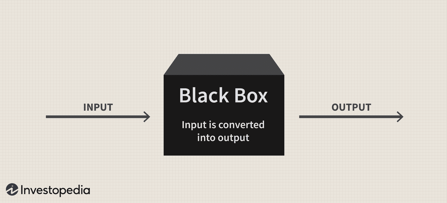 Figure 1: A black box does a bunch of calculations on the input \(x\), and then spits the output \(y\) out. Machine learning is about learning the black box itself given input/output examples \((x,y)\). Courtesy of Investopedia.
In general, we call the input/output example \((x,y)\) data, and a set of such examples a dataset. The data \(x\) and \(y\) could be literally anything. For example, \(x\) could be a combination of images, text, 3D scans, tables, etc. As for \(y\), it could simply be a label if it’s a classification task, or a number if it’s a regression task, but it could also be an image or a piece of text if it’s a generative task (e.g., ChatGPT, where the prompt is \(x\) and the image is \(y\)).
For starters, we will see how this works for binary classification, which is the simplest prediction task.
Binary classification
Let us consider binary labels +1 and -1 (the exact labels don’t matter). We consider a single real number as the output of the predictor \(f\). Precisely speaking, if \(f(x)\) is bigger than 0, then we predict 1 for \(x\), otherwise we predict -1. Pretty straightforward.
Let us consider a simple example. Let $x$ be the number of hours a student studies, and $y$ is whether the grade is pass or fail (pass = +1, fail = -1). Imagine we collected a bunch of data from past semesters on a tough course and get a silly histogram like this (the ASCII art is intentional; I want to emphasize the simplicity):
                                   + + +
                               + + + + + + +
                 - - - -     + + + + + + + + +
               + - - - - - + + + + + + + + + + +
           - - - - - - - + - - + + + + + + + + + + +
    0hrs -------------------- 5hrs -------------------- 10hrs
Let me tell you really quick what a histogram is. A histogram is a very useful graph for data visualization. It stacks the data points on top of each other within “bins”, where taller bins indicate higher frequencies. Here, a bin stands for a specific number of hours, but it can also stand for a range of hours to create a coarser graph so that the thinner the bins, the finer (but sometimes noisier) the histogram. Note that we have two kinds of bins, the + bins and - bins, which we stakc on top of each other. We are free to visualize our data in the way that makes most sense to us.
Ok, now let’s do machine learning. In the above histogram, most of the students who passed studied 5+ hours. Seems like 5 is the magic number; it’s a threshold that almost guarantees that the student will pass the course. Therefore, we can predict that a student will pass the course is they studied at least 5 hours and fail otherwise. We just did machine learning!
Indeed, what we did is machine learning at its most primitive level. We just plotted the data and figured out a pattern for passing the course.
Modeling the problem
Machine learning formalizes and generalizes this whole process. The mathematical modeling is to write down equations that describe your inputs and how they’re mapped into outputs. Machine learning is the science of figuring out the patterns. It’s often done with math because visualizing the data can only get you so far.
But why is it helpful? Suppose we want to predict whether a random future student will pass or fail given the number of hours they studied. Then, we can use a specific equation for predicting this. This has the benefit of being standardized, automated, scaled, and less prone to human error from visual interpretation. And when we talk about high-dimensional data, then visualization is out of reach, so machine learning becomes necessary to do any principled predictions.
Assumption 1: the data points are sampled “iid”
For example, in the above histogram, students who fail the course appear to have studied 3 hours on average, and 6 hours for those who passed. Conditioned on knowing the student’s passing grade, we can tell approximately how long they studied.
Let us take a random student from any past or future semester. We assume the relation between study hours and grade to have the same effect. This is a very important assumption in machine learning: we assume that our model will work in the future and will not drift. Roughly speaking, this corresponds to the assumption that students from all semesters have identical studying habits and behave independently from each other.
More precisely, we assume that the observed data points \((x_i, y_i)\) are iid (independent and identically distributed), and this is a crude assumption that statisticians and machine learning researchers love to use because it simplifies the math a lot. This is the first part of our mathematical model.
Of course, in practice, data can drift and what used to work may not work anymore. The simplest solution is to fit your model again on the new data. This is an important area of research and is related to model adaptation, which is the study of making models adapt to shifting data domains.
Assumption 2: study hours are normally distributed within each class
Students who passed seem to be randomly scattered around some average number of study hours. This is clear from the histogram.
When we say random, we usually think of the normal kind of randomness, the bell-shaped curve. The special thing about this curve is that it arises naturally when we average independent quantities. The variance/dispersion around the average decays exponentially as you go further. Due to its importance, I will dedicate a whole post to the normal distribution, but for now, just believe me that it is the most natural way to model the average of iid random variables (with unbounded support and bounded variance). In the above, we can ignore the lower bound of 0 hours and assume unbounded support. (It’s true that you can’t study negative hours, but you might slack so much that it would be like you’re un-studying.)
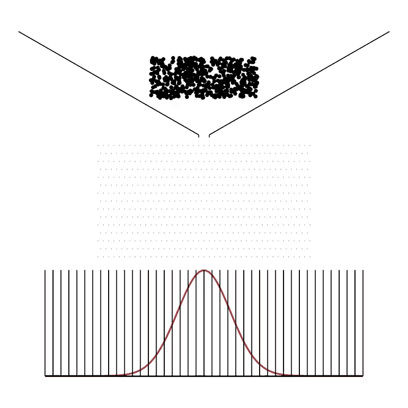 Figure 2: A galton board. The balls drop at the center, but shifts randomly every level, resulting in a histogram that converges to the normal distribution. Retrieved from this page.
This is the second part of our model. For a random passing student, we assume that the study hours are normally distributed around some average study time (and equivalently for failing students).
We can also use fancier distributions, but let’s stick to normal distribution with fixed variance. Note that this assumption does not meaningfully capture black-swan/long-tailed effects, such as the outlier student who passed with only 2 hours of study since the probability of that happening under our model could be extremely low (depending on the variance). Still, this model is good enough for our purposes. Such sacrifices are normal when modeling real-world problems, and keeping track of these modeling simplifications and discrepancies and knowing what to keep and what to leave is an important part of mathematical modeling.
The Resulting Model
Based on these two assumptions, we can find a closed form expression for the best threshold using maximum likelihood estimation (see below). If we further assume equal class priors and equal variance for the two bell curves, then the best threshold is exactly their midpoint. If you do the math, you will see that it is just \((6+3)/2 = 4.5\). This is almost 5, so our theoretical result agrees with our visual intuition.
Our prediction model under the two assumptions can be written as: \(f(x)\) = +1 if \(x > 4.5\), -1 otherwise. That’s pretty much it.
Model complexity
In practice, \(x\) may be complicated and not necessarily normally distributed, and the rule for predicting \(y\) may not be that simple.
For example, in surveys, there should be an upper limit on the number of study hours because students reporting an exorbitantly high number are lying to us, so we can deduce that they’re likely to fail. Math cannot elegantly capture this human intuition, but it’s a valid model. In that case, instead of using one threshold, we can use two! (Bet you didn’t see that coming.)
But what if the data is more complicated, and there are also outlier students with specific patterns for predicting their success? Should we add more thresholds?
As naive as a human decision can be in this scenario, this is one of the biggest conundrums of machine learning, and it’s often framed as a bias-variance trade-off. As we make our predictor more complex, we make it more susceptible to overfitting, i.e., fitting to noise or patterns that don’t exist.
Choosing the right complexity for the predictor is one of the main challenges in machine learning… or it used to, until deep learning came and gave us the middle finger. The classical Occam’s razor logic that “simpler” models are preferred over “complex” models does not really apply to deep learning models, at least not naively (probably because we’re not using the right model complexity measures; simple parameter count is a horrible proxy). Nowadays, deep learning models run efficiently on GPUs and scale up ad infinitum.
Deep learning is magical because its complexity adapts to the task. You could have the equivalent of a million thresholds for this silly prediction problem of pass/fail, yet a deep learning model—a neural network—can still find a solution that generalizes surprisingly well. To make things more confusing, the same model will gladly fit complete garbage random data perfectly, so it certainly can overfit if it wants to! How is this possible? Would you be surprised if I told you that nobody really knows? Nobody has a satisfying general explanation of this phenomenon. It’s sadly true, but it’s also exciting. This is one of the most interesting questions in deep learning, and we still don’t have a satisfying explanation. The explanation that I like is that this adaptive complexity comes from some “implicit regularization” of neural networks, but let’s keep that for another post.
Finding the model that fits
Once we define our prediction model, the process of fitting it to the data might not always be direct.
It is often not possible to directly optimize the fitting objective, e.g., the expected risk. One of the classic exceptions is linear regression, where the objective can be optimized directly and a closed form solution is attainable. Otherwise, we have to formulate a sound optimization problem that: 1) fits the model satisfactorily, and 2) can be solved efficiently.
The canonical example in deep learning is digit classification on the MNIST dataset. We minimize a loss function on MNIST (i.e., a measure of the discrepancy between a prediction and the ground-truth) and train a neural network with some optimizer (most likely gradient descent-based, such as SGD or Adam). We fit the model well enough (e.g., 98% accuracy) with an efficient algorithm (e.g., runs on one GPU in a few minutes).
Despite the simplicity above, problem formulation remains very important. However, the beauty of our modern models—those obscenely large neural networks—lies in their robustness to bullshit modeling. Namely, you can design all kinds of neural network pipelines for solving a bunch of complex tasks, and you can still mess up quite a lot and add unnecessary tricks without getting hurt by your own bullshit. At the end of the day, if your loss function is supposed to do something, and the algorithm is working, then your neural network is gonna do that thing and it will generalize well for you because it’s very kind to us sometimes, or as Noam Shazeer puts it: “we attribute their success, as all else, to divine benevolence”.
Nonetheless, it is important to understand that, despite the robustness of the neural networks, we still have to make sure that we are solving the right problem. Your loss function should make sense.
Regression
What if we want to predict the actual grade instead of pass or fail? Instead of \(y\) being -1 or +1, we want \(y\) to be a real number.
Let us consider the same data, but with actual grades instead. Here is an ASCII plot:
                                   7 8 9
                               7 7 7 7 8 8 9
                 3 3 4 4     2 7 7 6 7 8 8 8 9
               2 2 2 4 4 4 4 5 7 6 6 7 7 7 8 8 9
           1 2 6 1 2 2 3 5 5 8 6 6 6 7 6 7 7 7 7 8
    0hrs -------------------- 5hrs -------------------- 10hrs
Since the points have a numerical value, we can rely on the vertical axis to represent this numerical value to get a better visualization:
    9 |                                       1   1 1 1
    8 |                             1       1 2 2 2 1   1
    7 |                               3 2 2 4 1 2 1 1 1
    6 |               1               1 2 3   1
    5 |                         1 1 1
    4 |                     2 2 1 1
    3 |                 1 1   1
    2 |             1 1 1 2 1
    1 |           1     1
grade |    0hrs -------------------- 5hrs -------------------- 10hrs
The numbers represent the frequency of students who got that grade given the number of study hours (think of these as the height of 3D bins extending out of the screen, like a contour plot). We can see a clear linear trend: the number of study hours predicts the grade reliably, except for some outlier cases. In math, a linear equation is represented as \(\textsf{grade} = a \cdot \textsf{hours} + b\), where \(a\) and \(b\) are some numbers that we can figure out with algebra. That’s linear regression in a nutshell.
Binary Classification vs. Regression
[This section has some equations, which you can safely skip.]
It’s tempting to say that regression generalizes binary classification. Indeed, we can easily get +1 and -1 from a real number using a thresholding rule. In the above case, if a grade is 5 or more, it gets a +1. Otherwise, it gets a -1.
However, I will show you that the opposite is true in a deeper sense. Namely, I’ll show the counter-intuitive fact that binary classification can be at least as general a predictive framework as regression!
Classification > Regression?
First of all, the given data points in the above case are the number of study hours, usually called the regressor, input, or \(X\) (we use capital letter because it’s a random variable, i.e., not given). What we want to predict is whether a student passes or fails. What we want to predict is called the regressand, label, output, or \(Y\).
In the regression case, the predicted grade is \(\textsf{grade} = a \cdot \textsf{hours} + b\). What about binary classification? That’s the part where people jump to conclusion quickly and think of prediction in terms of bits. In learning theory / decision science, we represent a binary prediction as a probability:
\[\Pr[\textsf{pass} = +1 | \textsf{hours} = x],\]which is read as the “probability of passing given \(x\) hours of study” (we’ll skip \(x\) sometimes for clarity). Probabilities have values in [0, 1], but we can easily get -1 and +1 by thresholding at, say, 0.5. More generally, we can map a probability to the real numbers with the logit function: \(p \mapsto \log \frac{p}{1-p}\), and vice versa with the sigmoid function: \(x \mapsto \frac{1}{1 + \exp(-x)}\), so we’re not constrained to bounded values. Thus, the fact that binary classification is learning a conditional probability function under the hood changes the picture completely.
Instead of interpreting \(\textsf{grade} \implies \textsf{pass}\) as a conversion from a real number to a bit, we can also interpret it as a data generating process \(\textsf{pass} \implies \textsf{grade}\) relating uncertainty about passing to an observed grade. That is a very Bayesian way of looking at prediction. One could choose to view the grade as a rescaled belief/credence/probability of passing, say from 0 to 9. There is no one correct way; just different ways of looking at things and modeling them.
Ok, but how do we learn \(f(x) = \Pr[\textsf{pass} | \textsf{hours} = x]\), which would then give us \(\textsf{grade}\) after rescaling? Well, we could use logistic regression!
I bet you’re confused. Hear me out. The term binary classification is confusing. It’s true that we output a binary label, but the real part is classification because we actually never learn a binary function from data directly! Ok, rarely, not never. If you insist on learning an arbitrary binary function directly with no structure, you are basically memorizing a look-up table, which scales horribly. We almost always have missing data or noise in real-life, so probabilities come in for the rescue to represent those uncertainties.
Bayes Rule and Maximum Likelihood
So, how do we learn those “probabilities”? We use the celebrated Bayes rule:
\[\Pr[\textsf{pass} | \textsf{hours}] \Pr[\textsf{hours}] = \Pr[\textsf{hours} | \textsf{pass}] \Pr[\textsf{pass}].\]The unknown object of interest is \(\Pr[\textsf{pass} | \textsf{hours}]\), which is the prediction we want to make. We already have \(\Pr[\textsf{hours}]\) (well, not literally, but we have samples of hours in the data). Its exact value is not that important here as we’ll see. The probability \(\Pr[\textsf{pass}]\) is our prior belief in the probability of passing, which can be 0.5 for equal chances if no historical evidence is available.
Here comes the interesting one: \(\Pr[\textsf{hours} | \textsf{pass}]\). It is the distribution of study hours among students who passed, exactly what we were modeling earlier as normal distributions. When we write it down as a function of unknown parameters \(\theta\) (i.e., the mean and variance of the normal distributions) and fit it to observed data, we call this quantity the likelihood. In machine learning, the goal is to maximize this likelihood by choosing the best model of \(\Pr_\theta[\textsf{hours} | \textsf{pass}]\) with respect to model parameters \(\theta\). That’s the part where we have some leeway in modeling the data generating process. If we wear our Bayesian hat for a second, we can say that this probability is our uncertainty in the data generating process. The inherent randomness is aleatoric, and whatever randomness that comes from modeling is epistemic, i.e., it can be reduced with better knowledge.
So, in order to determine the best \(\Pr_\theta\), the most intuitive thing to do is to choose the probability distribution that maximizes the evidence we have collected based on the dataset. Precisely speaking, we choose the probability distribution parameters \(\theta\) that maximize the likelihood. That process is called maximum likelihood estimation (MLE), the foundation on which most machine learning models are based. The Bayesian upgrade to that is when we also plug in our prior beliefs on \(\Pr[\textsf{pass}]\), which would give us the maximum a posterior estimation.
Maximum Likelihood <=> Linear Regression
The canonical example that demonstrates the generality of classification and MLE is the following one. Let’s assume that: (i) the grades follow a linear trend, and (ii) the residual/vertical errors from that line follow a normal distribution. Then, MLE gives us ordinary linear regression exactly. See here, for example. Isn’t that amazing? I still feel amazed by this equivalence, and I think it’s one of the most beautiful results in machine learning.
There is no shortage of probability distributions out there, but the normal distribution is most likely all you need. In fact, many distributions are transformations of (a collection of) normal variables. Choosing the right distribution to model the randomness or uncertainty in the data generating process is an art that comes with experience. Recall the section “Modeling the problem” above and see whether the connection to process modeling makes sense or not.
Machine Learning in a Nutshell
Let me recap what machine learning is:
- Collect data from the real world.
- Model the data generation process. (Hint: you can model only the part required for predicting a bit.)
- Fit the model to the data.
- Predict the future with your model. (Hint: your prediction could be a bit or a full simulation.)
That’s basically it. Allow me to elaborate.
Collecting data is an extremely important part of machine learning. Some of the biggest AI companies focus solely on this part, and Big Tech are all doing it like crazy.
Next is the modeling part, which is an art that is learned from study, practice, and experience. It’s difficult to describe algorithmically and can be extremely varied in terms of what is being modeled, how efficient the model is, and how scientifically valid or mathematically rigorous. It usually requires translating your real-world problem to a mathematical model that is tractable, analyzable, and solvable with math.
Once we model the problem, we’re halfway there. After modeling comes the “solving”, which we also denote with fitting or training the model in machine learning. This is often exclusively the territory of optimization scientists. Machine learning engineers often do not touch this part and just use it as is. It’s difficult to make meaningful progress here because the simplest methods are robust and work remarkably well in practice (which is a bitter reminder for those doing research in optimization, including myself). Still, the line between research and engineering is a bit blurry in deep learning. Some very important tweaks and improvements come from a healthy mix between the two, for example, exponential moving average estimation in Adam and gradient orthogonalization with Newton-Schulz in Muon.
Finally, the prediction part is often assumed to be simple, which used to be very true since “predictions” are done constantly in modern training algorithms, i.e., models have to do a forward pass on the data, which is not necessarily required for simpler classes of (older) models. Nowadays, prediction—or inference as it’s usually called—is a whole science, especially for large language models. Depending on the model, the forward pass during model training can look very different in inference. Due to business needs, the forward pass during model inference is being pushed to be much more efficient. This is the part that happens where we chat with language models (i.e., there is no training happening during the chat).
Concluding Thoughts
What I love about machine learning is its broad applicability to solve many tasks in life using machines.
I mean, look at what machine learning models we have nowadays. Who knew, ten years ago, that machine learning would give us ChatGPT, Midjourney, and Veo?
Do you know what these language models are modeling? They are just modeling the next token (\(y\)) given a sequence of tokens (\(x\)), roughly speaking. Given a prompt, they predict the next token. And do you know how they predict the word after it? I kid you not, they just append the previous token to the prompt and—you guessed it—predict the next token. Yet here we are. These things work crazy well, and the funny part is, nobody fully understands why. I swear.
Looking at it more deeply, the goal of machine learning has always been broad, and it’s only natural that we got here. Machine learning has always tried to model the world, but we only model the parts that matter to us and only use models that are solvable or trainable with tractable algorithms.
I hope you enjoyed this high-level(-but-sometimes-has-math) post on machine learning. Let me know if you enjoyed it or have feedback. I’d especially welcome feedback from people coming from non-technical background.