Fenchel-Young Meets Donsker-Varadhan
In the last “X meets Y” battle, we’ve seen how a strong growth property of a function can be defined in two seemingly unconnected fields but end up being equivalent under the right assignment of objects. In this post, we will see the same phenomenon occurring for a fundamental variational/dual property, which is about the amount of “slack” left after removing a simple, constrained slice from a function.
FY
The Fenchel-Young inequality is one of the most beautiful and powerful inequalities in convex analysis.
Let’s quickly define the basics. A differentiable (because I’m lazy) convex function is a function \(f : \mathbb{R}^d \to \mathbb{R}\) such that for any vectors \(x, y \in \mathbb{R}^d\), we have
\[\begin{equation} f(x) - f(y) \geq \langle x - y,\, g \rangle, \qquad g := \nabla f(y). \tag{CVX} \end{equation}\]Put it simply, if you plot the function, then it should always be above its tangent. That’s convexity in a nutshell. You can go super fancy and rigorous with the details, generalizations, and extensions if you want, but I won’t.
But I’m afraid I have to… well, just a little bit.
Fenchel-Young (FY) inequality. The FY inequality simply says that, for any (not necessarily convex) \(f\) and its convex conjugate \(f^\ast\), we have
\[\begin{equation} f(x) + f^\ast(g) \geq \langle x, g \rangle, \qquad \forall x \in \mathbb{R}^d,\ g \in \mathbb{R}^d \tag{FY} \end{equation}\]Doesn’t it look kinda… hot? Ahem, I mean, it has this kind of symmetry + simplicity + depth, you know. But what is a convex conjugate in the first place? The FY inequality itself almost defines it:
\[\begin{equation} f^\ast(g) := \sup_x \, \{ \langle x, g \rangle - f(x) \}. \tag{Conj} \end{equation}\]In other words, the \(\sup_x\) part just gives the tightest \(f^\ast\) that satisfies (FY) pointwise, i.e., per \(g\).
Using \(g\) as the conjugate variable may not be standard, but I’m doing it here on purpose. If you were thinking: “\(g\) is often reserved for gradients, so this is confusing”, then you’re right because \(f^\ast\) is actually a function of gradient-like vectors rather than positions, i.e., vectors that lie in the conjugate space (where the conjugate space of \(\mathbb{R}^d\) is itself).
Intuition
These inequalities look opaque at first glance, but they do offer intuitive interpretations. The first intuition is mathematical, which is the right intuition in my opinion, and from which the inspiration for convex conjugacy is clearest. The second is geometric, which comes straight from visualizing the definition.
Mathematical intuition. Start by looking at (FY). Next, look at (CVX) and notice how the part that depends on \(x\) can be matched with (FY). Fix \(y\) and set \(g = \nabla f(y)\), then try to subsume the \(y\) part of (CVX) under the \(f^\ast(g)\) part of (FY).
\[f(x) + \underbrace{\langle y, g \rangle - f(y)}_{=\,f^\ast(g)} \geq \langle x, g \rangle.\]Define the quantity \(h(z;g) := \langle z, g \rangle - f(z)\), keeping this \(g\) fixed. By (CVX), \(h(z;g) \leq h(y;g)\) for every \(z\), so \(f^\ast(g) = \sup_z h(z;g) = h(y;g)\). This means that the convex conjugate is the smallest “offset” that makes (FY) hold for every \(x\) at a specific “slope”. This offset need not be positive as the nonnegative “slack”, or FY gap, is \(f(x) + f^\ast(g) - \langle x,g\rangle\). For differentiable convex \(f\), equality is available at every \(x\), attained exactly at \(g = \nabla f(x)\).
Not all convex functions satisfy (CVX) as nicely as you would like. You can always construct instances of convex \(f\) where convexity is just barely satisfied (like a constant function), but it’s more instructive to first study the nice ones to understand how convexity behaves. One particularly convenient class is differentiable strongly convex functions, where there is a nice degree of uniform strict convexity (the parabola is the canonical example). Now, given a specific gradient \(g\), the expression \(\langle z,g\rangle-f(z)\) defining the convex conjugate is uniquely maximized at the point on which \(g\) was evaluated. For example, if we know that \(g=\nabla f(y)\), then \(\nabla f^\ast(g) = \nabla f^\ast(\nabla f(y)) = y\), so the gradient of \(f^\ast\) is just the inverse map of the gradient of \(f\), i.e., \(\nabla f^\ast = (\nabla f)^{-1}\). Strongly convex functions demonstrate the operational meaning of \(f^\ast\) most clearly.
Geometric intuition. The geometric intuition comes from this Math StackExchange page. It provides a way to visualize the equation of the convex conjugate. I’ll just quote Julek’s answer here:
To me the best interpretation is economic. Interpret 𝑓(𝑥) as the cost to produce the quantity 𝑥 of some product and interpret 𝑦 as the market price per unit. Now notice that 𝑓∗(𝑦) represents the optimal profit at given prices 𝑦 . The quantity 𝑥𝑦 represents revenue from sales and 𝑓(𝑥) represents production costs.
Now for the geometrical interpretation. If you sketch the graph of the costs of production 𝑓(𝑥) and assume it convex, continuous, and differentiable, you will see that the point of optimal production, given prices 𝑦 , is given by 𝑦−𝑓′(𝑥)=0 , and this can be found graphically with a ruler, looking for the tangent in the cost curve with the same slope 𝑦 . If you place the ruler in that tangent point, it can be seen that the ruler intersection with the vertical axis will give −(𝑥𝑦−𝑓(𝑥)) .
This is a very useful calculating device. Provided only with the graph of 𝑓(𝑥) and a ruler, the analyst is able to turn the ruler and find what is the optimal profit for each possible price. This can be plotted into another piece of paper. Then given any price 𝑦 he is able to find what was the optimal profit. Without noticing, he has discovered the conjugate function.
The following figure is also taken from the same page, due to Dimitri Bertsekas from his lecture notes.
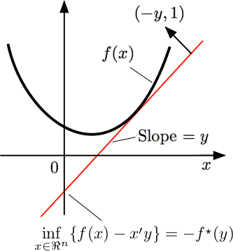
In general, I don’t like to interpret the values of $f^\ast$ themselves because they’re confusing. They’re literally the largest “difference” between \(f(y)\) and \(\langle y, g \rangle\) for each \(g\) (and the difference is not necessarily positive), and that’s what the definition says. In optimization, the role of \(f^\ast\) in (CVX), and hence in the duality gap and optimality certificates, is more useful than what the geometric interpretation alone offers in terms of intuition.
DV
I first saw Donsker and Varadhan’s Variational Formula on Wikipedia while looking at some properties or proofs of KL divergences. Same as before, when I looked at the formula, I immediately thought: “that’s just a convex conjugate but for distributions”. Here is an excerpt from the Wikipedia article linked above.
Donsker-Varadhan (DV) Variational Formula.
Let \(\Theta\) be a set endowed with an appropriate \(\sigma\)-field \(\mathcal{F}\), and two probability measures \(P\) and \(Q\), which formulate two probability spaces \((\Theta, \mathcal{F}, P)\) and \((\Theta,\mathcal{F},Q)\), with \(Q \ll P\). (\(Q \ll P\) indicates that \(Q\) is absolutely continuous with respect to \(P\).) Let \(h\) be a real-valued integrable random variable on \((\Theta,\mathcal{F},P)\). Then the following equality holds \(\log \mathbb{E}_P[\exp h] = \sup_{Q\ll P} \{ \mathbb{E}_Q[h] − \mathbb{D}_{\mathrm{KL}} (Q \, || \, P) \}.\) Further, the supremum on the right-hand side is attained if and only if it holds \(\frac{Q(d \theta)}{P(d \theta)} = \frac{\exp h(\theta )}{\mathbb{E}_{P}[\exp h]},\) almost surely with respect to probability measure P, where \(\frac{Q(d \theta)}{P(d \theta)}\) denotes the Radon-Nikodym derivative of \(Q\) with respect to \(P\).
For simplicity, I’ll assume \(h\) is bounded and measurable, with \(P\) fixed and the sup over probability measures \(Q\).
I initially saw the following potential correspondence from the formula above:
\[\begin{align*} \mathbb{E}_Q[h] &\to f(Q) &&? \\ \mathbb{D}_{\mathrm{KL}} (Q \, || \, P) &\to \langle \frac{Q(d \theta)}{P(d \theta)},\, Q \rangle &&? \\ \log \mathbb{E}_P[\exp h] &\to f^\ast(h) &&? \end{align*}\]But it’s not quite there; the conjugate variable is not clear from this attempt, and the signs look wrong. The sup already has the form of (Conj), but we just need the right assignments.
Quick detour, sorry
Let’s first look at a beautiful form of FY. Let \(\rho\geq0\) be a density w.r.t. \(P\) such that \(\int_\Theta \rho dP = 1\). I’ll write \(H\) for negative entropy throughout. Define the functionals:
\[L(h) = \log \int_\Theta \exp (h) \, dP, \quad\text{and}\quad H(\rho) = \int_\Theta \log (\rho) \rho \, dP,\]where we set \(0\log0 := 0\). These are just the functional forms of the LogSumExp and negative entropy functions, and if you know a bit more about them, you’ll know that they are the convex conjugates of each other under the inner product:
\[\langle h, \rho \rangle_P := \int_\Theta h \rho \, dP,\]so FY would imply that
\[\int_\Theta h \rho \, dP \leq H(\rho) + H^\ast(h),\]where \(H^\ast\) is the convex conjugate of \(H\), i.e., \(H^\ast = L\). A direct proof is surprisingly simple and uses Jensen’s inequality. The above inequality and the proof can be found in this Math StackExchange post.
Entropy and relative entropy
There is entropy, and there is relative entropy. Well, relative entropy is just KL divergence:
\[\mathbb{D}_{\mathrm{KL}} (Q \, || \, P) = \int \log\frac{dQ}{dP} dQ.\]Writing the densities \(p=dP/d\mu\) and \(q=dQ/d\mu\) w.r.t. a common measure \(\mu\), we get the well-known decomposition (for finite terms):
\[\mathbb{D}_{\mathrm{KL}} (Q \, || \, P) = \int q\log q \, d\mu - \int q\log p \, d\mu = H_\mu(q) - \mathbb{E}_Q [\log p].\]Here \(H_\mu\) is negative entropy measured against \(\mu\). The term \(-\mathbb{E}_Q [\log p]\) is also called the cross-entropy loss (assuming \(Q\) is the data distribution and \(p\) is the learned density).
The density \(\rho\) in the previous section was defined w.r.t. \(P\) itself, so setting \(\rho = dQ/dP\) gives
\(H(\rho) = \int \log(\rho)\rho\, dP = \int \log \frac{dQ}{dP} \, dQ = \mathbb{D}_{\mathrm{KL}}(Q \, \| \, P).\) So our negative entropy \(H\) (or \(H_P\)) was already relative entropy! The choice of reference measure \(P\) matters a lot here; this isn’t the same functional as \(H_\mu\), and the choice of density \(\rho = dQ/dP\) is also necessary.
To summarize, we have that the negative entropy of the derivative \(dQ/dP\) w.r.t. \(P\) is equal to the relative entropy of \(Q\) w.r.t. \(P\), i.e., \(H_P(dQ/dP) = \mathbb{D}_{\mathrm{KL}}(Q \, \| \, P)\).
Back to DV
Now set \(\rho=dQ/dP\) in the conjugate formula and look at what happens:
\[\begin{align*} H^*(h) = L(h) = \log \mathbb{E}_P[\exp h] &= \sup_{Q\ll P} \{ \mathbb{E}_Q[h] − \mathbb{D}_{\mathrm{KL}} (Q \, || \, P) \} \\ &= \sup_{\rho} \left\{ \int h\rho\,dP - H(\rho) \right\} . \end{align*}\]It’s quite clear now, isn’t it? This was just entropy-based conjugacy in disguise! And the implicit object we’re optimizing over is precisely \(\rho\), i.e., the Radon-Nikodym derivative \(dQ/dP\). The sup over \(\rho\) is such that \(\rho \geq 0\) and \(\int \rho dP = 1\).
Let’s take a closer look at the conjugate definition behind FY and the DV identity
\[\begin{align} f^\ast(g) &:= \sup_x \, \{ \langle g, x \rangle - f(x) \}, \tag{FY} \\ H^*(h) &= \sup_\rho \{ \langle h,\rho\rangle_P - H(\rho) \}, \tag{DV} \end{align}\]so we have the correspondence
\[\begin{align*} f &\longrightarrow H \\ f^\ast &\longrightarrow H^\ast = \log \mathbb{E}_P[\exp (\cdot)] \\ \langle g, x \rangle &\longrightarrow \langle h,\rho\rangle_P = \mathbb{E}_Q[h] \end{align*}\]which elegantly completes the correspondence between DV and FY.
FY = DV
The DV variational formula isn’t just analogous to a convex conjugate, it is, in fact, one. The function and its conjugate are the negative-entropy and LogSumExp, with \(P\) being the fixed reference everything is measured against.
Observe again from the above that \(x \in \mathcal{X}\) corresponds to \(\rho \geq 0, \int \rho dP = 1\) (equivalently, \(dQ/dP \geq 0, \int dQ = 1\)). On the other hand, the conjugate variable \(h\) corresponds to \(g \in \mathcal{X}^\ast\). Recalling the equality condition quoted in the excerpt \(dQ/dP = \exp(h)/\mathbb{E}_P[\exp h]\), we observe the same story as \(\nabla f^\ast(g)\) recovering the optimal \(x\) where, ideally, \(g=\nabla f(x)\).
Indeed, differentiating LogSumExp at \(h\) gives precisely the softmax of \(h\), which is the optimal density \(\rho = \exp(h) / \mathbb{E}_P[\exp (h)]\), with P as the reference measure. The optimal measure \(Q_h\) is obtained by tilting \(P\) by \(\exp(h)\) and renormalizing.
So the conjugate-gradient-as-inverse-gradient story is still there because differentiating \(L(h)\) gives the optimal density \(\rho\), and differentiating \(H(\rho)\) takes us back to \(h\) plus an additive constant. Since \(\nabla H(\rho) = \log(\rho) + 1\), we have that \(\nabla L(\nabla H(\rho)) = \rho\) but \(\nabla H(\nabla L(h)) = h - L(h) + 1\). The constant is fine; adding it to h changes nothing after applying softmax because softmax is shift-invariant. Equivalently, we can write \(\rho = \exp (\bar{h})\) and \(\bar{h} = \log \rho\), where \(\bar{h} := h - L(h)\).
Finally, writing the full FY gap in the DV case gives a particularly nice form:
\[\mathbb{D}_{\mathrm{KL}}(Q\|P) + L(h) - \mathbb{E}_Q[h] = \mathbb{D}_{\mathrm{KL}}(Q\|Q_h) \geq 0.\]This is the nonnegative “slack” from the FY story, and it vanishes exactly when \(Q=Q_h\).